The official version of this document can be found via the PDF button.
The below content has been automatically generated from the original PDF and some formatting may have been lost, therefore it should not be relied upon to extract citations or propose amendments.
Stewarts' Response to the Scrutiny Review of the Draft Damages (Jersey) Law 201-
About Stewarts
Stewarts is an international litigation firm specialising in complex high value disputes. Our practice areas include Personal Injury, Clinical Negligence, International Injury and Aviation.
Within these practice areas, the claims we undertake exclusively relate to injuries of the utmost severity or death. Our specialisms are recognised by top-tier rankings in the leading legal directories, Chambers, the Legal 500 and the Times.
Whilst there are many firms of solicitors which do some complex and high-value personal injury litigation, we are one of very few firms in the UK that exclusively specialise in such claims and do not conduct claims relating to non-disabling injuries (aside from the rare scenario when there are secondary claimants involved in the same incident as a claimant with severe injuries). We are well-placed to provide a response to this consultation, as almost all our cases involve issues surrounding periodical payments orders and the inevitable contrast with a lump sum award applying the discount rate. We acted for the Claimants in a number of the leading cases concerning periodical payments[1] and concerning negative discount rates in Bermuda[2].
We take the opportunity to point out that we are a relevant stakeholder for this review on the basis we have and continue to represent a number of Jersey based clients and this review, together with this response, are made in their interests. We work in conjunction with Jersey co-counsel David Benest at BCR Law in representing our Jersey clients.
Julian Chamberlayne, Partner and Head of International Injury acted for the plaintiff, in the case of X v Estate of Y (Deceased) & oths heard in the Royal Court of Jersey, Samedi Division (2013/143), a polish citizen injured in a road traffic accident in Jersey. We were able to obtain the first PPO in Jersey in this case.
In addition, we have two current catastrophic injury cases running in Jersey[3] in which our expertise is required to ensure those clients have the best chance of obtaining the correct level of compensation.
Accordingly, our submission has a particular focus on the impact of the issues raised by this review on those with seriously disabling injuries, with reference to those Jersey cases mentioned above.
We attach the following documents to assist in interpreting our comments below:
- The Discount Rate – a report for the Ministry of Justice prepared by Paul Cox, Richard Cropper, Ian Gunn and John Pollock. Dated 7 October 2015;
- PFP – MoJ call for evidence; and
- Stewarts Discount Rate Calculation example.
Wells v Wells approach and ILGS
It is accepted within the Draft Damages (Jersey) Law ("Draft Law") that Jersey's courts have generally adopted English common law'.
In our view, the English common law approach determined by the House of Lords in Wells v Wells remains the fairest and best way of meeting the full compensation principle.
In his leading speech in the House of Lords, Lord Lloyd of Berwick stated that the judges in the three jointly heard cases of Wells:
"were right to assume for the purpose of their calculations that the plaintiffs would invest their damages in I.L.G.S. for the following reasons:
- Investment in I.L.G.S. is the most accurate way of calculating the present value of the loss which the Plaintiffs will actually suffer in real terms.
- Although this will result in a heavier burden on these defendants, and, if the principle is applied across the board, on the insurance industry in general, I can see nothing unjustNo doubt insurance premiums will haveto increase in order to take account of the new lower rate of discount
- The search for a prudent investment will always depend on the circumstances of the particular investor. Some are able to take a measure of risk, others are notStill less is it his duty to invest in equities and gilts in order to mitigate his loss.
- How the plaintiff, or the majority of plaintiffs, in fact invest their money is irrelevant. The research carried out by the Law Commission does not suggest that the majority of plaintiffs in fact invest in equities and gilts but rather in a building society or a bank deposit"
The Wells approach was validated by the Judicial Committee of the Privy Council in Simon v Helmot with Lord Hope explaining at paragraph 47 that:
"finding a solution today is not so dependent on surmise and speculation as it was when the issue was being discussed in those cases three decades agoThe investment scene has been radically altered. The breakthrough came with the introduction of ILGS and the appreciation that there was at last a tool that could be used to provide protection against inflation. It is tailor-made for investors who want a safe investment for the long term. In practical terms that is risk free. As nearly as possible, it guarantees the availability of the money to meet costs as and when it is required. It may not be perfectBut it is the best tool that is available."
In the Draft Law, in line with the Ministry of Justice's (MoJ) 2017 consultation paper, a heavy emphasis is placed on investment return and investment risk. However, as Lord Hope's explanation suggests, the impact of inflation is equally as important. One of the reasons for adopting ILGS as a proxy return on which the discount rate should be derived was the difficulty courts otherwise faced in predicting future inflation. In the Court of Appeal case of Helmot, Sumption JA (as he then was), commented, stating at paragraph 38:
"The reason for calculating a lump sum award on the footing that the lump sum will be invested in index-linked gilts is that it achieves an automatic adjustment for future increases in the general level of prices."
The MoJ's 2017 consultation was right to acknowledge that it is essential for the discount rate to be set in a manner that fairly represents the 100% compensation principle. This echoes the MoJ's 2013 consultation on discount rate where it was noted at paragraph 6 of that paper that:
"if the rate is too high, the burden would fall on the victims of the wrongful act, who include some of the most vulnerable members of society, who would be under- compensated, thereby possibly increasing their reliance on the state and, therefore increasing costs to the taxpayer."
Underlying that observation and the points made by Lord Hope in Wells is the simple concept that the cost of meeting the long-term losses and needs of those seriously injured by the wrongful acts of another party may fall to a combination of the following:
- The injured party;
- The party who caused the injury or more commonly their insurer; and
- The State/taxpayers.
It is clearly appropriate for the party who caused the wrong, creating the loss, to be responsible for the financial consequences. Where those losses continue into the future, the resultant financial risk as to how those losses should be met in the long-term should be borne by the wrongdoer. There is no sound argument in principle as to why either the loss or the risk of meeting the long-term needs should fall to the injured party or to the State/taxpayer, unless of course the State is the wrongdoer.
The adoption of a discount rate based on ILGS does not lead to the single Claimant being "over compensated". Rather, Claimants may choose to take investment risks so as to attempt to improve their financial position. To require them to do so, however, as is contemplated by this Draft Law, would make them the only class of investor required to take risk so as to advantage some other party (the wrongdoer/the wrongdoer's insurer). This cannot be considered either fair or just. In reality most seriously injured Claimants base their decisions on investing their damages around meeting their disability needs and very few seek to take investment risks to outperform their needs.
Proposed Statutory Discount rates of +0.5% and +1.8%
We strongly oppose the introduction of statutory discount rates, to be set at +0.5% and +1.8%, because such rates would not satisfy the full compensation principle and the basis for proposing those rates is inherently flawed. The key reasons why we are of this view are:
- reliance on the model portfolios from GAD report 2017;
- emphasis on the investment decisions assumed to be made by individual Claimants;
- allowance for investment management charges and tax;
- The proportion of claimants who will be under compensated utilising a mixed portfolio approach is inconsistent with a full compensation regime;and
- The dual rate split: the Ontario Model and earnings related model.
- Reliance on themodel portfolios from GAD report 2017
The Draft Law relies on the GAD report 2017 which followed the 2017 MoJ consultations; we refer to our 2017 consultation response to the MoJ which has been provided with this response.
The MoJ asked the Government Actuary Department ("GAD") to analyse two model portfolios based on unpublished anecdotal reports of claimant investor behaviour. Portfolio A was considered to reflect typical low-risk' claimant behaviour, whereas Portfolio B was the highest end of the low-risk' spectrum. They were not asked to and did not analyse the lowest end of the spectrum. Therefore, not only are the conclusions on which the MoJ proposes this legislation is passed derived from an unpublished and small evidential base, they also do not reflect the full range of claimant investor behaviours.
Additionally, the low-risk' categorisation of the portfolios modelled by the GAD is disputed on the grounds that both models carry a serious risk for the claimant's ability to achieve full compensation. According to the GAD model, Portfolio A had just 5% invested in ILGS (with 46% in equities or alternative investments) and this figure was only 3% in Portfolio B (with circa 65% in equities or alternative investments). In contrast, the majority of the 2015 MoJ expert panel (the full report has been provided alongside this response) described the low-risk portfolio approach as one in which at least 75% of the portfolio is allocated to ILGS.
In preparing this response we have sought the views of 2 of the authors of that expert report: Richard Cropper and Ian Gunn. They have confirmed that they stand by the view that no account was taken of the fact that any claimant investment behaviour was in light of the need to hedge mortality risks, the impact of having insufficient capital following the purchase of a property (due to the Roberts v. Johnstone approach to future accommodation giving rise to a capital shortfall), earnings (rather than price inflation), taxation and active investment charges.
Personal Financial Planning (member of the MoJ's expert panel) have repeatedly warned that if one is to take account of real-life experience, that must be in respect of both claimants' liabilities to real earnings growth, taxation and investment charges, as well as the return on investing in a mixed portfolio.
By only looking at what claimants invest in and not why they are forced to invest in those assets, the discount rate is bound to be set at too high a rate, as claimant will have to invest with exposure to even more risk to cover real earnings growth, taxation and investment charges.
- Emphasis onthe investment decisions assumed to be made by individual Claimants
The House of Lords in Wells v Wells, as followed by subsequent courts who have considered the issue of whether ILGS is the best tool by which discount rate could be determined, have renounced the proposition that it was based on how Claimants choose to invest their compensation. The utilisation of ILGS as the benchmark is only ever a pragmatic proxy for the net real rate of return. It created a fair and predictable method by which future losses could be calculated that was not reliant upon expert evidence. It did not require speculation about the composition of any investment portfolio, the returns on the portfolio, the level of charges of investment managers and stockbrokers, the level of taxation nor a prediction of future inflation.
An individual Claimant's decision to take an investment risk is clearly their choice and a matter only for them. If their investments go well and they out-perform the discount rate, then their financial position is enhanced. However, that is as a result of the investment decisions/risks they choose to take after the conclusion of their case, coupled with the good fortune of those investment risks working out in their favour. If a Claimant who makes numerous risk-based investments were to achieve poor returns or actual losses, it would result in a performance below the discount rate and ultimately lead to compensation running out during his or her lifetime. There is nothing in law, currently, which would allow for him or her to return to the Defendant who caused their injury to seek further compensation. Once again, this potential outcome is a consequence of the risk the Claimant chooses to take in relation to any investments. The law should not be constructed in such a way that either forces the Claimant to take those risks, or requires them to do so for the benefit of the party who caused their losses in the first place.
We endorse the following points made by Personal Financial Planning[4]: that in their experience Claimants (1) do not invest in risk assets with the aim of maximising returns in order to generate over compensation that they can spend on wants' rather than needs', and (2) sometimes accept risk in order to facilitate the maintenance of their needs over time, often having also looked at family support to create a saving on care costs, state support and compromising or foregoing needs.
- Allowance for investment management charges and tax
It is essential to make full allowance for administration, management expenses, investment advice and the costs of purchasing and selling investments (both initial costs and subsequent changes). The need for such adjustments have been consistently acknowledged by GAD and the MoJ, but the level of the adjustment has not yet been determined nor applied to the modelling conducted by GAD.
Our Mr Chamberlayne, in his role as Chairman of the Forum of Complex Injury Solicitors (FOCIS) has been gathering data on this point from UK firms who regularly act as Deputy and/or Professional Trustee for seriously injured Claimants who have received substantial damages awards. We append a summary of the preliminary conclusions of an analysis of that data by Ian Gunn of PFP as recently submitted to the MoJ and GAD. The broad indication from that data is that overall costs, including investment advice, tend to fall in the range 1.5% to 2%. This is materially higher than the 0.5% figure tentatively suggested by GAD in their 2017 report for the MoJ. It is within, but at the upper end, of the range the GAD referred to in their 2018 report to the Scott ish Parliament. Note that this data did not include the impact of tax on the investment return, as that impact varies considerably between Claimants based on their personal circumstances, but GAD accept that a further adjustment for tax is necessary. This may be achieved in crude terms by rounding up rather than down, until someone conducts the research to enable a more informed adjustment to be made.
In this summary Ian Gunn adds:-
"I should point out that the costs set out above are incurred by claimants in managing cash flows and risk, selecting what to buy and what to avoid, when to sell, holding and keeping track of investments, the income they generate, capital gains and capital losses, and all regulatory compliance. They are not performance fees, i.e. payments to an investment manager in the expectation of achieving superior returns compared to a benchmark, so that the investor ends up better off than without active investment management".
It is essential that the adjustment for all aspects of investment management charges and tax is made to ensure the resultant discount rate reflects the likely net return that these Claimants will achieve on a low risk basis. The alternative is that the law would need to be changed to make such costs a recoverable head of damages. However we contend that is a less satisfactory approach as it will inevitably lead to disputes in many claims.
- The proportion of claimants who will be under compensated utilising a mixed portfolio approach is inconsistent with a full compensation regime
As strong advocates of the Wells v Wells approach, we are of the opinion that the assumed investment risk profile of the Claimant should be assumed to be that of very risk averse or "risk free".
These issues were previously considered and addressed in a 2015 expert report commissioned by the Ministry of Justice. The appointed panel of experts, consisting of Paul Cox, Richard Cropper, Ian Gunn and John Pollock, came to the majority view that the discount rate should continue to be based on the Wells approach. The panel cautioned that if the approach of a mixed portfolio balancing low risk investments were to be taken (category b), then only up to 25% of that portfolio should be allocated to non- risk-free assets. The modelling also demonstrated that if the approach were adopted, the discount rate would be 0%.
The majority of the panel did, however, emphasise that having reviewed Dr Cox's research on the modern portfolio theory, the emerging risk measures appeared to be inconsistent with the requirement for the portfolio to be considered very low risk. This analysis highlights the very significant deviations that could arise even with a low risk or very low risk mixed portfolio. They could cause a significant proportion of Claimants to be undercompensated and hence leave them unable to meet their needs.
In the Bermuda case of Thomson v Thomson and Colonial Insurance Company Limited, similar issues can be described as having arisen. At first instance in the Supreme Court of Bermuda, Chief Justice Kawaley observed at paragraph 38 that the case appeared to be the first occasion in which a common law court has been required to consider, in the future damages discount rate assessment context, the respective merits of an assumed investment of the entire lump sum to be awarded in ILGS as opposed to in a mixed basket of investments. The Defendants in that case had relied on the expert evidence of
a Canadian Actuary, Christopher Gorham, who advocated a mixed portfolio moderated with what he described as a "safe fund". This was similar in concept to the financial economics approach that is advocated by Dr Cox and considered by the other members of the Ministry of Justice's expert panel back in 2015. This mixed portfolio was also broadly comparable to the "low risk" portfolios that feature in the GAD 2017 report to the MoJ. At paragraph 93 of the Thomson Judgment, it was observed that Mr Gorham: "conceded under cross-examination by Mr. Harshaw that on his investment model between 50 and 33% of plaintiffs would not have sufficient funds. He viewed his approach as fair to both claimants and defendants."
Chief Justice Kawaley commented:
"I viewed his approach as a stunning dilution of the prevailing legal policy preference, in the future loss discount rate calculation context, for a hypothetical investment in an instrument likely to generate a risk-free rate of return."
At paragraph 100, Chief Justice Kawaley also made reference to the evidence of the Claimant's Actuary, (former Government Actuary), Christopher Daykin, as follows:
"As Mr. Daykin explained, institutional investors are able to safely invest in a wider range of investment instruments because they are investing on behalf of multiple ultimate investors whose needs to redeem their investments stretch out over multiple lifetimes. Such investors are also able to hedge against short-term risks in ways which are generally impossible for the typical individual personal injury Claimant. I find that there is a fundamental distinction between the investment goals of the hypothetical prudent investor, especially an institutional investor, (who is not investing sums received by way of compensation for tortious injury), and the investment goals of the hypothetical prudent plaintiff. As regards the latter, there are explicit legal policy imperatives which require the courts assessing the appropriate level of lump sum to award to:
- assume that the least possible risk will be taken when the lump sumis invested by the prudent Claimant with a view to achieving the goal of full compensation;
- ignore the commercial realities of how lump sums may actually be invested; and
- utilize tools for the calculation of the discount rate which are sufficiently simple to be conveniently deployed both in the context of assessing damages in and out of court without the need for the expense of expert evidence save in exceptional cases."
The Bermuda Court of Appeal subsequently fully endorsed the Judgment of the Chief Justice.
At paragraph 23, Bell JA commented further that:
"What Mr. Daykin was saying is essentially that Mr Gorham's theory of sufficiency demonstrated that, using his model, there is approximately a 50% chance of a Claimant receiving a fund sufficient to meet expenses and losses, with the other side of the coin being that 50% of Claimants would not have sufficient assets to do so. Consequently, Mr. Daykin concluded that these figures come nowhere near meeting the principle of full compensation which has been accepted over many years by the courts. What Mr. Daykin said in relation to the 90 to 95% figures was not that these represented over- compensation on the basis of the Chief Justice's ruling, but that if one were to test a model proposed in place of the Wells mechanism (as advocated by Mr Gorham), then
there would have to be a demonstration that the payments were sufficient for the Claimants in at least 90 to 95% of cases in order to come close to providing full compensation."
The Ministry of Justice's expert report in 2015 does not appear to have directly addressed the question of sufficiency, this being the percentage of Claimants who would, under the alternative portfolio models proposed by Dr Cox, end up with insufficient assets to meet their future needs. However, reading between the lines in relation to the panel of experts' comments concerning the similar concept of deviation, a significant proportion of those Claimants would end up with insufficient funds. This no doubt led the majority of the panel to come to the conclusion that it was an inappropriate way for calculating the discount rate.
In the GAD 2017 report they acknowledged that the need for the MoJ to consider the issue of what level of under compensation was acceptable within a full compensation regime then make any necessary adjustment to the figures derived from their modelling before setting the discount rate. This issue was echoed in the Justice Committee's Report, published 30 November 2017, in particular paragraphs 22 -24.
The sufficiency question was posed by us to Wrigleys Solicitors and Fensham Howes, firms which routinely advise Claimants on long-term investment following the resolution of their litigation. They both indicated that when considering low risk investment portfolios for their seriously injured clients, they tend to strive for a sufficiency ratio of 90 to 95%. In doing so, they take account of the life expectancy risk to try and ensure that Claimant funds would last to the upper end of the range of probable ages. Fensham Howes' approach to investment is based upon years of research which has repeatedly shown that the perfect investment offering both low price volatility and high long term returns above inflation does not exist.
Due to the boom and bust cycle of the economy the uncertainty caused by this lack of stability means that if a Claimant is in need of funds when the market is low, it will adversely affect his remaining award to his/her detriment and could therefore leave them reliant on the state when the money runs out. This volatility, as outlined in the expert report prepared for the Ministry of Justice in 2015, creates a sequencing risk "which occurs where one year of below RPI investment returns is immediately followed by another, which is immediately followed by another etc. Poor investment return sequences combine with portfolio withdrawals in a highly destructive way because more fund units need to be enchased [sic –encashed] to generate the same annual income. The double erosion of capital following a market fall -the market drop and the drawing an equal income at depressed fund value -is what makes sequencing risk potentially destructive One of the lessons of the technology boom and bust followed shortly by the financial crisis was the importance of the order, or sequence, of extreme investment returns. If a sequence of market drops means the capital of a fund is 50 per cent lower than planned, a 100 per cent gain is needed to return the fund to where it should be"[5]
- The dual rate split: the Ontario Model and earnings related model
The Draft Law refers to the UK GAD's analysis and proposes Jersey statutory discount rates of +0.5% up to 20 years and +1.8% applicable to all the years where the loss is deemed to be for a period of over 20 years. The proposed rates and the use of a form of the Ontario model, in splitting periods, lacks adequate supporting analysis for either the 20 year period or the proposed rates. We understand that the 1.8% discount rate is a hybrid of Portfolio A and B over 30-50 year period but we strongly believe this is flawed for two reasons. First, claimants are likely to have a shorter investment life than a composite of 30-50 years. The only claimants that would have an investment life of that length of period would be minors. Since the beginning to 2016, only 3% of Stewarts' PI cases involved minors, therefore the assumption regarding investment period is inappropriate. Secondly, as discussed above, the Portfolio A and B contain 46% and 65%, respectively, in equities and alternatives and therefore cannot be considered a sufficiently low risk portfolio appropriate for claimants. Furthermore, if the Draft Law were passed as proposed, it appears that a Claimant with a loss spanning 19 years would receive more compensation that one of a little over 20 years, as evidenced below:
That is clearly perverse.
We contend that the more important issue is there are to be differential discount rates is to provide full compensation for earnings-related heads of future loss, notably loss of earnings and future care and case management. It is also applicable to other earnings- related heads of loss, such as the cost of a Professional Deputy and medical professionals including therapists.
The impact of earnings inflation and the need for an adjustment has already been closely scrutinised and accepted in the context of a periodical payment regime as reflected by the Court of Appeal Judgment in Flora v Wakom (Heathrow) Limited and Thompstone v Tameside. This has resulted in the general practice thereafter being to apply ASHE 6115 indexation to PPOs for care and case management and less frequently, other earnings- related indices for other earnings-related losses.
The application of this adjustment to lump sum compensation has been considered by the Guernsey Court of Appeal (in the highly regarded Judgment) of Sumption JA (as he then was) and the Privy Council. It has also been considered by the Chief Justice of Bermuda, and subsequently endorsed by the Court of Appeal in Bermuda in Colonial Insurance Company Limited v Thomson (conjoined with Harvey v Warr en).
Lord Hope in the Privy Council Judgment concerning Helmot v Simon quoted favourably from the Judgment of Sumption JA as follows:
"if an adjustment could be made which would serve to compensate the respondent more exactly for his losses there was no legal reason why it should not be made" (paragraph 40) and "having considered the evidence, Sumption JA said that it seemed to him to constitute strong unchallenged evidence of both the existence of a gap between price and earnings inflation in Guernsey of the order of 2%, and the likelihood that over time it would persist" (paragraph 41).
"As for the question whether there should be more than one rate this seemed to him to be correct in principle in a case where there was a significant difference between elements representing loss of earnings and care costs" (paragraph 42).
Lord Hope's conclusion, strongly supported by Lord Brown at paragraph 75, was that: "75. if this Claimant is compensated for future loss only on the basis or projected RPI inflation, his award (intended to compensate for increased future losses over the period for his predicted further lifespan of 40 years) will almost certainly prove inadequate to meet his long-term future care needs.
- The real question in the Appeal must therefore be this: Which approach is preferable: one which ignores the established claim showing an increase in real earnings and so produces an award of almost certainly less than will be sufficient to meet the Claimant's likely future care costs, or one which uses the best available evidence
- The answer must therefore be obvious."
Lord Brown at paragraph 82 referred to Sarwar v Ali and oths in which Lloyd Jones J accepted what he described (at paragraph 143) as:
"A consensus between the experts that the RPI is not an appropriate index for Periodical Payments in respect of future loss of earningsThe same is true of the future cost of care and case management."
Finally and pithily from the Helmot Judgment, Lord Dyson at paragraph 113 said:
"There can be no justification for holding that, on these admittedly bare and rather crude facts, damages should be assessed using a discount rate based on RPI inflation. Such an assessment would be bound to lead to under-compensation."
In Sarwar v Ali & the MIB, the Defendant did have an Economist, a Mr Cooper. At paragraph 142 of the Judgment, Lloyd Jones J stated:
"there is near unanimity on the part of the experts in relation to certain of the issues. Dr Wass (Economist), Mr Hogg (Accountant), Mr Copper (Economist) and Mr Hall (Accountant) all agree that average earnings generally increase at a faster rate than prices, that on the balance of probabilities average earnings growth is likely to exceed growth in prices in the future and that, on the basis of historical data, linking Periodical Payments to loss of earnings for RPI would be very likely to undercompensate the Claimant."
At paragraph 161, he observes that:
"She (Dr Wass) concludes that all the measures of earnings growth which she examines exceeds the corresponding measures of growth in pricesShe concludes that measures of earnings growth in the care sector have consistently exceeded the growth in aggregate earnings over the period 1998-2005."
The Judge then quoted from the evidence of the Claimant's Accountant, Mr Hogg, which had confirmed that:
"For the whole period 1963-2006 earnings (AEI) increased on average at 1.9% per annum faster than prices (RPI) but over the last 20 years the rate increase has been lower at 1.53% above price inflation as mentioned by RPI."
The Judge noted at paragraph 163 that:
"Mr Cooper and Mr Hall agree that there is a longstanding pattern showing average earnings rising faster than price inflation."
At paragraph 166 Lloyd Jones J dismissed one of the Defendant's counter-arguments, being:
"wholly unpersuaded by Mr Cooper's arguments based on the possibility of improved productivity in the provision of care for the Claimant in the future."
He observed that was not supported in any way by the care experts.
As can be seen, when this issue has been closely analysed by the courts, the evidence in favour of making an adjustment for earnings-related heads of loss was on each occasion considered overwhelming and required to achieve full compensation. The evidence demonstrated that the scale of the adjustment required tended in the long-run to be between 1.5 and 2%. This would mean it is necessary for there to be a differential earning related discount rate that is between 1.5 and 2% lower than the general (prices) discount rate. This would ensure that the full compensation principle is adhered to and avoid manifest unfairness, notably to those Claimants for whom a Periodical Payment for those heads of loss was wholly unavailable, not offered by the Defendant, or not appropriate for a variety of other factors.
We note that there has apparently been a more modest earnings inflation differential in Jersey in recent years. The short timescale for responding to this consultation has meant we have not been able to scrutinise that phenomenon. It conflicts with the economic evidence advanced in all of the above mentioned cases concerning negative discount rates in Guernsey, Bermuda and Jersey[6]. However, rather than having this issue prescribed by primary or secondary legislation, we propose that the Courts be given a broad discretion to set a differential earnings related discount rate, if the evidence supports such a conclusion. This would be in line with the approach to the issue of the indexation of periodical payments for earnings related losses pursuant to the Damages Act.
Reverting to the concept of the different rates for different periods of time, our position is that we do not consider that to be either necessary or appropriate. We observe this concept was carefully considered and dismissed by the Ministry of Justice's panel of experts, with them commenting at their paragraph 6.7 that they were:
"not persuaded that the discount rate needs to vary by term of loss at the current time, if the discount rate was set by reference to ILGS alone, as the real interest rate yield curve is relatively flat over the long durations."
Fensham Howes, Financial Investment Advisers, emphasise that the risks Claimants face vary with investment time horizon, but do not inevitably, let alone predictably, reduce. For investors with short time horizons, volatility is the greater problem and this leads the prudent advisor to recommend portfolios with little or no volatility risk. Such portfolios will by nature contain a high proportion of low risk fixed income securities and will therefore have very limited potential for real growth above inflation. For investors with long investment time horizons, protecting against inflation is usually the greater problem.
The only common law Judgment which we are aware of in which an adjustment to the discount rate was varied by the term of loss is the Hong Kong case of Chan Pak Ting v Chan Chi Kuen et al. The Defendants in their above-mentioned Bermuda case of Thomson v Thomson and Colonial Insurance Company Limited urged the Bermuda Court to take a similar approach. It was a path adopted by the Defendant's Actuary, Christopher Gorham. However, as Chief Justice Kawaley in Thomson observes at paragraph 34:
"Chan Pak Ting must be understood in the context of its facts. There was a joint expert report and it was common ground that the ILGS measure was inappropriate as it was not even a potentially available instrument vehicle for the hypothetical reasonable Hong Kong Plaintiff. The vehicles taken into account were not selected as a more appropriate reference tool than ILGS but merely as the best available measure. The Hong Kong Court clearly considered the measures available as a "next best" rather than a "preferred" option."
A statutory introduction on Periodical Payment Orders in Jersey
In England and Wales, the Courts are required to consider, in all cases, whether to make a PPO. The Court can order a PPO even if the Claimant prefers a lump sum, where it is deemed to be in the Claimant's best interests (Sarwar v Ali & the MIB). Our experience is that virtually all UK insurers predominantly negotiate on a lump sum basis, often under Part 36 Civil Procedure Rules, carrying costs consequences for Claimants in failing to accept and fail to beat that offer. Many Claimants, who would prefer PPs, at least for future care, are often forced to settle on a lump sum basis as they are never given a PP based offer.
We fully support the introduction of PPO availability in Jersey, however the power to set the indexation applied to any PPOs should lie with the Courts. Leaving the power in secondary legislation, as is suggested in the Draft Law, is far too crude a measure, which risks falling out of step with use of PPOs. It is far more appropriate to grant the Courts wide discretion so that submissions can be made in individual cases insuring that the Claimants are fully compensated.
The Courts having the discretion to bespoke indexation of a PPO was crucial in the case of X v Estate of Y (Deceased) & oths, in which we represented the Plaintiff. If the PPO indexation had been set by secondary legislation, the PPO would have been entirely inappropriate considering that the Plaintiff is a Polish national who had returned to reside in Poland and consequently faced future losses that were not likely to rise in line with the Jersey economy.
Furthermore, if the indexation of PPOs were to be set by secondary legislation, it is not clear which index would be chosen. There appears to be three main options, being:
- Price indices, which we argue does not adequately reflect the overall economic trend to be suitable as the set benchmark for all heads of loss types;
- Jersey earnings indices, which is based on a relatively small group and also may have a high earner skew (due to the socio-economics of the jurisdiction), which may be unsuitable as a bench mark for carers earnings; or
- English indices, which are based on a sufficiently large sample group benefitting from the wealth of data from ONS as set out in the ASHE tables, notably those related to the earnings of carers. Thisis particularly important as the care claimis usually the largest head of future losses for those with serious injuries. If the indexation is inaccurate then over time the PPO will not provide for the cost of the claimants care claim and that phenomenon will compound year on year.
As shown in the above example, the setting of any of the above indices across the board would be inappropriate and would not sufficiently cater for all heads of losses. This issue is far better left to the judges to apply on the facts and evidence in each case, albeit as with the common usage of the ASHE 6115 index in England, it is likely that a few early court decisions will then establish a commonly applied norm.
What we would like to see in relation to the statutory discount rate?
It is our proposal that the annual revision of the discount rate follows a pre-established formula averaging the real yields on ILGS over the preceding 12 months. The new rate would then simply need to be published/announced by the Government Actuaries. A prescribed formula would remove the danger of subjectivity and personal views of the individuals otherwise chosen to set the discount rate, some of whom may be subject to pressures from different lobbying groups.
A broader review should be conducted by a panel of independent experts. The Government Actuary, acting on the advice of an expert panel, in order to set the differential rate for earnings heads of loss and, if necessary, report to the States of Jersey on any issues that warrant a change to the methodology concerning the discount rate.
We consider that the use of the Ontario model, splitting years and applying arbitrary rates to these periods should be avoided.
If the proposed assumed rate of return on a "low risk" portfolio is taken into account when setting the discount rate and a higher discount rate consequently applied, Claimants will be forced to take risk to overcome these issues. It is also unclear how you calculate the net return on alternative assets without basing data on past performance or simulated past performance which is neither reliable nor compliant with the FCA COBs 4.6.7 - 4.6.9.
We invite the States of Jersey to follow the decisions of the Privy Council in Helmot v Simon, the Bermuda Court of Appeal in Colonial Insurance Company Limited v Thomson and the PPO cases of Thompstone v Tameside and Sarwar v Ali & the MIB. This would allow a differential discount rate for earnings-related heads of loss, notably future losses for care and case management and loss of earnings, to reflect the real and very longstanding differential between pay and earnings inflation which has been variously put in the range of 1.5 - 2%.
We acknowledge that the Draft Law proposes the introduction of 0% floor to the discount rate. While we are not strongly opposed to this, we would like to see this implemented only in relation to price based heads of loss, with the courts being granted discretion to make further adjustments as is necessary, e.g. for cases involving earnings heads of loss, foreign nationals and other such differentials. Implicitly, this would mean departing from the aim of full compensation, which we contend the States of Jersey should not do absent the clearest of evidence and compelling policy reasons.
If notwithstanding all of our submissions the States of Jersey remains minded to pass legislation as contemplated by the Draft Law, it is essential that the rate does not depart from the full compensation principle and does not result in a significant proportion of Claimants going under compensated with the result that their damages run out during their life time. The consequence of this is Claimants would be unable to meet their injury related needs and fall back on the state for support. If this approach is to be taken then we invite the States of Jersey to apply the appended methodology when determining the discount rate(s) to be set. You will see that, using the GAD's highest return on RPI+1%, the result would, on our analysis be, a discount rate of -2.75% for prices related heads of loss and of -4.5% for earnings related heads of loss. If the 0% floor is to be implemented, that would obviously override and so the before mentioned rates would not be considered. However, what this does illustrate is the implausibility of setting a positive discount rate while succeeding in upholding the long established 100% compensation principle.
Julian Chamberlayne
In the event of any queries, please contact Julian Chamberlayne via email at jchamberlayne@stewartslaw.com
 Stewarts Law
Solicitors
5 New Street Square
London
EC4A 3BF
For the attention of Julian Chamberlayne
23rd October 2018
Your ref: Our ref: IGG
Dear Julian
MoJ call for evidence: summary of responses by FOCIS member firms
Thus far, you have received responses from seven firms providing professional deputyship/trustee services to clients with personal injury awards. The responses provide information about the cost of investment, including financial advice, investment management, transaction costs, custodianship and collective fund management costs.
The evidence shows a clear and unsurprising inverse relationship between investment costs and the amount of capital invested. In other words, as a percentage of the capital invested, investment costs decline as the amount of capital invested rises.
Five of the firms provided anonymised data about 98 individual clients, with a total reported value of a little under £120 million. One firm provided aggregate data for 31 clients, with a total value of £30 million, and aggregate data for a further 100 portfolios but without quantifying their value. Therefore, there is data for 129 clients with a total value of around £150 million. The average portfolio in the sample is £1.16m.
The first observation to be made is that, on average, these portfolios are significantly larger than those modelled by GAD for the MoJ. For the latter, GAD was instructed to model portfolios to provide for a loss of £10,000 per annum for 30 years (therefore £300,000 +/- depending on the discount rate applied). Averaging the cost data provided in the sample is therefore bound to understate the real-world cost for such an assumed claimant, and this is an important caveat to the comments overleaf.
Respondents indicated that:
• Annual fees for independent financial advice to manage cash flows and overall risk parameters were largely in the range 0.25% to 0.75% of the capital invested, with the majority in the middle of that range, i.e. around 0.50%. These fees are exempt from VAT.
• Some respondents use individual discretionary fund managers to construct a tailored portfolio, with or without an IFA. Their reported fees range from 0.85% to 1.0% plus VAT (1.02% to 1.20% including VAT). Additional costs with discretionary fund managers include: custody fees, internal (in-house) fund costs, market transaction, brokerage and third - party costs. Some of these are paid per transaction and some as a percentage of value. The data is very noisy' and no meaningful average can be calculated for these additional costs, although some allowance for them is necessary. IFA fees are additional, as above.
• Alternatively, respondents use collective investment fund managers with advice from an IFA. Fund management fees range from 0.5% to 1.5%. Additional costs with investment funds include custodianship, audit, accountancy and fund administration. The overall cost figure for collective investments tends to fall in the range 1.0% to 1.5%. No VAT is charged on these costs or fees. IFA fees are additional, as above.
• Platform fees are reported in the range 0.1% to 0.3% depending on the value of the portfolio. No VAT is charged on these fees.
• There are outliers above and below the ranges referred to, as would be expected in such a small sample size and with a diverse population of clients.
The broad indication is that overall costs, including advice, tend to fall in the range 1.5% to 2%. I should point out that the costs set out above are incurred by claimants in managing cash flows and risk, selecting what to buy and what to avoid, when to sell, holding and keeping track of investments, the income they generate, capital gains and capital losses, and all regulatory compliance. They are not performance fees, i.e. payments to an investment manager in the expectation of achieving superior returns compared to a benchmark, so that the investor ends up better off than without active investment management. This is often what conventional' investors are seeking, although on average they are unlikely to achieve it. This is a crucial distinction when considering the real world that claimants have to inhabit when exposed to investment risk.
Yours sincerely

Ian Gunn Consultant
2
Adjustments for consideration in setting the discount rate
Step 1: Estimated annual investment rate of return1 1.00%
Adjustment to account for possiblity that 10% of claimants
Step 2: will be under compensated2 -1.50% Step 3: Adjustment for investment management fees and tax3 -1.75%
Adjustment to account for differences between UKRPI and
Step 4:
JRPI -0.50% Discount Rate for price related heads of loss -2.75% Step 5: Adjustment for earnings inflation[1] -1.75% Discount rate for earnings related heads of loss -4.50%
*Please note that even making the above assumptions claimants are still exposed to other risks including: risk that inflation may actually be higher (as only a very limited proportion of the model low risk Portfolios are inflation linked assets); the longevity risk that they may outlive their life expectancy; risk that their needs worsen; the risk that RPI is not representative due the nature of goods required for their specialist needs; and currency risk.
1RPI+1%, chosen as it is the highest return analysed in the GAD report 2017. 2from figure 1 (page 3) of the GAD report 2017. From that graph, this is the
discount rate that would result in roughly 10% under compensation risk with reference to Portfolio A. Therefore adjustment is the difference between +1% (our assumed nvestment return) and -0.5% (the discount rate that ensures only 10% undercompensation risk) = +1.5%
3Based on our initial analysis conducted with PFP (please find appended). Taken the midpoint between 1.5% - 2%.
The Discount Rate
A report for the Ministry of Justice
Prepared by
Paul Cox,
Richard Cropper, Ian Gunn &
John Pollock
7 October 2015
This report has been prepared within the context of guidance provided by the Ministry of Justice on the parameters within which the advice has to be provided. The authors can provide more extensive comment and advice if this is considered helpful.
The content of this report is the considered opinion of the authors but, for the avoidance of doubt, does not necessarily represent the opinion of any professional bodies or working parties where the authors are fellows, members or participants. In particular any input made to this report by Dr Pollock cannot be assumed to be necessarily reflective of the opinions of the Institute and Faculty of Actuaries or the Ogden Working Party.
AUTHORS
Dr Paul Cox is Senior Lecturer of Finance at Birmingham Business School, University of Birmingham and an Investment adviser at The National Employment Savings Trust (NEST). Since 2007 he has provided pension and investment expertise to the Department of Work and Pensions, the Personal Accounts Delivery Authority, and the Department for Business, Innovation and Skills. Paul has been involved in drafting several government consultations on pensions and investments and recently authored reports include Helping consumers and providers manage DC wealth in retirement' (2015) and Metrics and models used to assess company and investment performance' (2014). Prior to academia Paul was a fund manager at Kleinwort Benson and RCM Global Investors. He has been a representative on many regulatory and institutional investment working groups. He's currently a chief examiner of higher level practitioner examinations at a large chartered professional body.
Richard Cropper and Ian Gunn are consultants at Personal Financial Planning Limited, a company of Independent Financial Advisers dedicated to advising recipients of personal injury damages. Richard and Ian provide post-settlement advice on investment planning and management of personal injury damages, personal injury trusts, State Benefits entitlement, statutory provision of care and assistance, taxation and assurance. In addition, they both provide pre-settlement expert opinion on form of an award' issues (periodical payments or lump sum). Richard provided expert financial advice for the claimants in all four of the Thompstone et al indexation of periodical payments' cases, which have been pivotal in changing the damages landscape in favour of periodical payments in maximum severity.
Dr John Pollock is a Consulting Actuary. He has a background in institutional investment management and within the University sector but has specialised for the last 20 years in providing expert evidence in the UK Courts on a range of matters where actuarial input is required. He has been the representative of the Institute and Faculty of Actuaries on the Ogden Working Party' since the publication of the 4th edition of the Actuarial Tables with explanatory notes for use in Personal Injury and Fatal Accident Cases (the Ogden Tables') in 2000. He was recently involved in drafting the Actuarial Professional Standard X3 : The Actuary as an Expert in Legal Proceedings.
- The current legal framework and a reworking of the past approach in current economic circumstances.
- A review of actuarial practice in setting discount rates more generally.
- What is the appropriate measure of inflation?
- A financial economics approach to the discount rate.
- Should discount rates vary by duration of loss?
- Summary and recommendations.
Appendices
- Sources of data and evidence used.
- A financial economics approach to the discount rate – an expanded discussion.
- Trigger for review.
Set out below is a list of the issues the panel of experts has been asked to consider, cross- referenced to the relevant section(s) of our report.
Requirement | Chapter(s) |
The types of investment suitable for a personal injury claimant of the type envisaged by the law relating to the setting of the discount rate who is in receipt of an award of damages for future loss caused by personal injury | 1,2,3,4 |
The risks attached to investments | 2,3,4, Appendix 2 |
If more than one type of investment is considered suitable, the balance or mix of these investments that should be made by the claimant | 4, Appendix 2 |
The rate of return that each of these types of investment could reasonably be expected to produce, what assumptions apply to these rates of return (including assumptions about the economic cycle and economic outlook), and how those rates of return are calculated | 4, Appendix 2 |
Whether, and if so to what extent, these results depend on the amount of the lump sum to be invested, or on the period for which the investment is expected to be needed | 5 |
Whether more than one rate should be set | 5 |
What specific data and evidence sources were used to calculate the proposed discount rate, and why these are the right sources compared to other alternatives | 1, Appendix 1, Appendix 2 |
The specific methodology applied to calculate the proposed discount rate, including any assumptions about inflation, tax and investment management and administration expenses | 1,2,3,4, Appendix 2 |
For how long a period the rate of return proposed would be expected to remain an accurate indication of the rate of return to be taken into account under section 1 of the Damages Act 1996 and whether (and if so how) the length of that period could be affected by setting a different rate | Appendix 3 |
The balance between simplicity of administration of a rate and the accuracy of the rate | 6 |
The current legal framework and a reworking of the past approach in current economic circumstances
- The function of this report is to assist the Lord Chancellor, and his counterparts in the devolved administrations, in their review of the responses to the first of the two consultation papers issued by the Ministry of Justice in 2012 and 2013. The first was entitled Damages Act 1996: The Discount Rate and how should it be set. 1 The second was entitled Damages Act 1996: The Discount Rate - Review of the Legal Framework. 2
- The review of these consultation responses, this report and other investigations that are deemed necessary, will assist the Lord Chancellor, and his counterparts in the devolved administrations, in their decision making about at what level the discount rate (or rates) should now be set, how the rate (or rates) should be calculated and what circumstances should trigger future reviews.
- The Ministry of Justice has provided us with copies of the responses to the first consultation paper. Our brief review of these responses is summarised in Appendix 1 to this Report.
 In England and Wales the Lord Chancellor has the power to prescribe the discount rate to be used in cases of personal injury and fatal accidents under Section 1 of the Damages Act 1996. More than one discount rate can be set and the Courts retain
1 Ministry of Justice. (2012). Damages Act 1996: The Discount Rate. Available:
https://consult.justice.gov.uk/digital-communications/discount-
rate/supporting_documents/discountratedamagesact1996consultation.pdf. Last accessed 19th May 2015. 2 Ministry of Justice. (2013). Damages Act 1996: The Discount Rate. Available:
https://consult.justice.gov.uk/digital-communications/damages-act-1996-the-discount-rate-review-of-
the/supporting_documents/damagesact1996discountrateconsultation.pdf. Last accessed 19th May 2015.
[1]flexibility to diverge from the prescribed rate should they be persuaded that the circumstances of the case merit such a departure.
- Our instructions are that the report content is to be framed with the context of the first consultation exercise. This is the approach to the setting of the discount rate within the prevailing legal framework. We cannot comment with authority on the legal issues involved but summarise for completeness and ease of reference our lay understanding of these main principles below.
- We are grateful for the guidance provided to us by the Ministry of Justice who have in turn sought advice from Counsel.
- The decision in 1998 by the House of Lords in the conjoined cases of Page -v- Sheerness Steel, Wells -v- Wells and Thomas -v- Brighton Health Care Authority 3 detail the background to the current legal framework adopted by the Courts in the UK. The decision of their Lordships was followed in principle by the Lord Chancellor in 2001 when he exercised his power under Section 1 of the Damages Act 1996 and set the discount rate at 2.5%. There has been no variation in the rate since this time. The Lord Chancellor had the power to set more than one rate, but declined to do so. The legal issues considered in Wells have been revisited in a more contemporary financial environment in the Judgment of Sumption JA in the case Helmot -v- Simon heard in the Guernsey Appeal Court, and the subsequent appeal of the decision in this case to the Judicial Committee of the Privy Council. [2] 5 The principal investment related issues which arose from consideration of these various cases can be summarised as follows.
• The purpose of assessing the amount of a lump sum award as compensation for future financial losses is to place the claimant into, as far as is possible, the same financial position as if he had not been injured. In Wells, Lord Steyn referred to the "100% principle", i.e. that the victim is entitled to be compensated as nearly as possible for all future losses.
• The availability of Index-Linked Government Stock (ILGS) enabled the Court to consider a theoretical framework within which a claimant could invest in a portfolio of ILGS which, if held to redemption in an adequately structured portfolio, would provide for the future losses or costs as they fell due, without risk of erosion through inflation (to the extent the loss in future would have moved from current levels in line with the RPI, the basis of indexation of ILGS), or loss of capital. The availability of ILGS then provided the most accurate way of assessing the value of future losses in real terms (at least relative to RPI inflation).
• The claimant is not an "ordinary investor" in the sense of being able to wait for long-term returns to materialise, or to ride-out volatility in asset prices.
• The claimant may choose to invest in other securities offering the promise of higher rates of return but this is not relevant to the calculation of lump sum damages. Consideration of what is actually done with an award, how it is spent or how it is invested is not to be taken into account.
• A notional annuity' approach is envisaged with income from the lump sum award being drawn annually with an additional on-going diminution of capital, this being exhausted over the expected period of loss (itself a function of life expectancy).
• Simplicity of calculation of the discount rate and relative infrequent adjustment to the rate was seen to be desirable.
• An investment in equities was deemed inherently risky. Expenses to meet a future loss for a claimant could not be deferred until financial markets recovered (if they had fallen). Lord Hope noted in Wells that there could be no question about the availability of the money when the investor requires repayment of capital and there being no question of loss due to inflation'. It was noted in Wells that insurers and pension funds invest in ILGS to meet index-linked liabilities. Such action was deemed prudent'.
- Our subsequent review of investment alternatives to ILGS in Chapter 4 is framed with these clearly stated constraints in mind. This is the basis of our instructions.
- Our additional instructions are that neither general improvements in living standards nor qualitative improvements in an element of the claimant's loss over time are relevant to the Lord Chancellor's task of setting the discount rate. We are therefore instructed not to take these matters into account. The consequences of this constraint on our advice and opinions is considered in Chapter 3 where measures of inflation are reviewed.
- Given the requirement for this review of investment alternatives to be made within the current legal framework it seems appropriate to review how the Lord Chancellor set the rate in 2001 and to consider what discount rate (or rates) would now result from a comparable analysis being undertaken at the present time.
- In Wells -v- Wells their Lordships considered average gross ILGS yields over one and three year periods and made a pragmatic reduction for taxation, as a claimant investor bears taxation on income payable from ILGS. At the time the Judgment was made the average net annual ILGS yield (in excess of inflation) was around 3% and the conjoined cases were decided based on multipliers calculated at this rate. What this implied in practice was that if the award of damages was calculated using a 3% discount rate, and the claimant then invested in ILGS securing such a rate of return (if he desired to do so), then the "100% principle" would have been met.
 The Lord Chancellor sourced ILGS yields from the Bank of England Debt Management Office for the three-year period to June 2001. The rationale behind Lord Irvine's decision is reproduced in Appendix A.1 of the first consultation paper referenced above. Additional insight is gained from the comments of Baroness Scotland in the House of Lords debate on the matter on 29th November 2001. In brief terms, Lord Irvine used a three-year average of those ILGS yields with over five years to maturity. The resultant figure was 2.46%.6 A 15% reduction for tax was deemed appropriate giving a yield of 2.46% – 0.37% = 2.09%. The discount rate was then set at 2.5%. What can be seen is that the Lord Chancellor followed the precedent set in Wells and set the rate with reference to ILGS, but it is known that he additionally considered returns on other securities to be relevant, together with the interests of claimants and those of defendants more generally. The authors presume this further review, beyond the largely arithmetic exercise of calculating and then referring to average net ILGS yields, was reflected in the rounding upwards' decision that was made in 2001. The authors note that only the interests of claimants are deemed
6 Although in a document entitled "Damages Act 1996: Briefing Note on Index-Linked Gilt Average Yield Calculation (Data Issues)", dated 6th July 2001, written by the UK Debt Management Office (DMO), obtained by PFP under a Freedom of Information Request, the DMO confirms that their calculation of the yield on all index-linked gilts for the three years up to and including 8th June 2001 was 2.61%. This was said to be based on the following assumptions:
• All IGs were used in the calculation, with no adjustment for the near maturity portions of IGs close to redemption, the rump stock, or WI stock;
• Daily data yield observations;
• Simple average;
• The use of the standard market convention of a 3% inflation assumption in the calculation of real yields from prices.
This figure was then adjusted to 2.50% for various technical reasons and corrections.
[1]relevant in Wells, the impact of any decision about the discount rate on defendants was not deemed relevant.
- The Courts have the power to use a different discount rate, or rates, if they can be persuaded that the features of the case justify a departure from the rate set by the Lord Chancellor. The authors are aware of a number of cases involving non-resident claimants 7 and are also familiar with the reported decisions in a number of cases considering changes in economic circumstances more generally 8 and where periodical payments are not available. 9 The Courts have not yet used a rate other than 2.5% in circumstances where the Damages Act 1996 applies, although they have in jurisdictions where the Act does not apply and when assessing future losses in cases not necessarily involving injured persons. [2]
- Before reworking the analysis made in 2001 in the context of current economic circumstances it may be helpful to detail some of the basic features of ILGS.
• ILGS offer coupon payments and redemption proceeds that are linked to the Retail Price s Index (RPI). There has been some debate over whether Consumer Price s Index (CPI) linked ILGS should be issued in future but none have been issued to date.
• The substantially greater part of the return from ILGS comes from the return of indexed capital. In recent years stocks have been issued with trivially small coupons (as low as £1/8 p.a. per £100 nominal). A claimant investor would be taxed on income but not on gains in capital.
• The ILGS market is both substantial and liquid. There are securities with redemption dates ranging from 2016 to 2068. The crude average future term is c21 years.
• There are two types of security, those with an eight-month lag in indexation and those with a three-month lag. For practical purposes this can be ignored. The actual level of future inflation is essentially irrelevant; ILGS protect again inflation as measured by the RPI.
- The graph below shows the three-year moving average of yields on ILGS securities with over five years to maturity (as were considered by the Lord Chancellor in 2001). [3] Figures are publicly available for 0% and 5% inflation assumptions (only relevant for the lag') and the 0% figures have been used below. The differences are not material, as noted above.
 Gross over 5 year ILGS yields - 1 and 3 year averages
3.00
2.50
2.00
1.50
1.00
1 year 0.50
3 year 0.00
-0.50
-1.00
- Current and historic average real yields are noted in the table below.
Term | Current Yield | 1-Year Average Yield | 3-Year Average Yield |
0 to 5 years | -0.73% | -1.02% | -1.31% |
Over 5 years | -0.84% | -0.73% | -0.30% |
All stocks | -0.83% | -0.74% | -0.32% |
- The graph shows quite clearly that there has been a marked decline in ILGS yields since 2001, when the current 2.5% discount rate was set. This is an investment phenomenon that has not been confined to the UK. In the US real yields on Treasury Inflation Protected Securities (TIPS) currently average 0.7% [4] and in the Eurozone real yields on inflation-protected securities are 0.1%. [5] The lower ILGS yields in the UK relative to yields available on inflation protected securities in the US and Europe may be explained, at least in part, by the basis of indexation, being the RPI in the UK and CPI measures in other countries. Inflation measures are discussed in more detail in Chapter 3.
- This is to be expected. Real yields will be higher when economies are experiencing growth in real terms and demand for credit is high, and will be low in periods of weak economic growth when consumers and businesses focus on saving, not consumption. The pace of the decline in ILGS yields accelerated after the financial crash in 2008. Those wishing to invest conservatively have had to accept lower rates than in the past.
A Report by the International Monetary Fund contains a useful summary of trends in
this regard. [6]
- Although opinions can differ on the matter, from an economic perspective one might expect the real yields on ILGS to reflect investor opinions on likely real economic growth in the UK (or real yields in other countries to reflect likely real economic growth in those countries). Government debt has to be financed and repaid from taxation revenue, which is a function of economic activity.
- Anticipated levels of real economic growth have implications for anticipated levels of earnings growth relative to inflation. One would expect real earnings growth to be high when real economic growth is high (which in turn would most likely be associated with higher levels of real yields on ILGS) and real earnings growth to be low when real economic growth is low (which in turn would be most likely associated with lower levels of real yields on ILGS).
- The issue of the appropriate levels of inflation to consider in this exercise is discussed in Chapter 3. In this discussion we are mindful that our instructions are that neither general improvements in living standards nor qualitative improvements in an element of the claimant's loss over time are relevant to the Lord Chancellor's task of setting the discount rate. The discount rate is, put simply, the return after tax and management expenses relative to inflation', whatever that might be considered to be.
- A further consideration mentioned by their Lordships in Wells was the fact that a lump sum award based on a discount rate calculated with reference to ILGS would most closely match the outcome for a claimant in respect of a Periodical Payment Order (PPO). At the time of Wells these could only be arranged by consent (this situation still prevails in Scotland, Guernsey, Jersey and the Isle of Man) but since the Courts Act 2003 the number of PPOs established, primarily for care costs, has grown significantly. If there is to be consistency between those cases settled by means of a PPO and those cases settled by means of a lump sum, then the purchase of a portfolio of ILGS might be considered to most closely replicate the expected PPO cash flows (setting aside for the moment the issue of the measure of PPO indexation, which now conventionally departs from RPI).
- If the current Lord Chancellor were to replicate the analysis made by his predecessor in 2001, then:
• The starting point would be the historic average of over five year ILGS yields.
• This is -0.30% over a 3 year period or -0.73% over a 1 year period.
• A modification then needs to be made for tax on the (indexed) coupon payments. The tax burden will vary from claimant to claimant, and their Lordships in Wells and, subsequently the Lord Chancellor, took a broad brush approach to solving this problem by simply reducing the prevailing gross real yield by 15%, suggesting a reduction to the gross yield at the time of 0.37%. The change in yields since 2001 and steady issuance of more securities with lower coupons complicates matters. The deduction for taxation will be modest. Time constraints have not allowed us to consider the issue of taxation in detail and for practical purposes we would suggest that this issue can be addressed in the rounding aspects of the calculation.
- The calculations outlined above suggest that the discount rate in current circumstances, if set using exactly the same methods used by the Lord Chancellor in 2001, would be between -1% and -0.5% depending on the allowance for taxation and the averaging period being used. From an actuarial perspective, the one-year average is considered to be more appropriate, and the panel is in agreement that rounding should be to the nearest half-percentage rate for use in the current Ogden Tables. On this basis, the discount rate would be -1%.
- A practical consideration which merits comment is that the ILGS market extends at the current time to 2068, a period of 53 further years. At the time of the decision in Wells the ILGS market extended for 31 years to 2030 [7]. This period of 53 years exceeds the life expectancy of many claimants (those in their early to mid-thirties in normal health) but is less than the life expectancy of some young claimants (if they have average life expectancy, although many do not). Life expectancy at birth is now around 90 years and this is an effective upper bound on the duration of losses likely to be considered by the UK Courts. The concept of discount rates trending towards an ultimate forward rate' features in insurance applications as will be discussed in the following chapter. Currently, nominal discount rates used for terms beyond those available in the conventional gilt market are somewhat higher than those at the longest available terms. This might suggest use of a modestly higher discount rate to apply to cash flows in the very longest tail of the spectrum being valued. The issue of different discount rates for different terms of loss is discussed in Chapter 5.
- A focus on ILGS returns can however hide more subtle features of the problems under consideration. If an award of damages is calculated at, say -0.5%, and a claimant invests in ILGS of approximate terms securing a net yield of -0.5%, then he would be fully compensated, but only to the extent that the heads of claim being valued will increase in future in line with the RPI. Chapter 3 will discuss whether claimant inflation is indeed properly estimated by the RPI or if alternative measures are more appropriate. These would impact on the discount rate assessed solely by an inspection of ILGS yields. Put crudely, if a head of claim was expected to grow faster than RPI in future then use of an ILGS based discount rate would overstate the discount rate, leading to under-compensation, and vice versa. To the extent that low real interest rates may be predictive of weak economic growth, and hence earnings growth, this issue may be of less importance than at times in the past when real interest rates were higher.
A review of actuarial practice in setting discount rates more generally
- The assessment of the present value of future earnings, care costs, services or pension rights is fundamentally an actuarial exercise. The Courts now accept this and the Actuarial Tables with explanatory notes for use in cases of personal injury or fatal accidents (known as the Ogden Tables') [1] are widely used by the Courts in the UK when making future loss calculations. In England and Wales they are admissible in evidence by virtue of Section 10 of the Civil Evidence Act 1995 and they are universally applied in other legal jurisdictions in the UK. This was not always the case. [2]
- The essentially actuarial aspects of the matter are, firstly, that the expected duration of
the payments being valued is a function of the projected mortality experience of the claimant (which varies by both age and gender) and, secondly, that the future payments require to be discounted' for accelerated receipt. The future payments are generally predictable' in real, inflation adjusted, terms and the discount rate is chosen accordingly. This means the Courts can conveniently make their calculations in current money' terms, the impact of inflation' being disregarded. Comparable calculations are made by actuaries in a large range of commercial applications, pricing insurance contracts, valuing pension liabilities and in all reserving and solvency assessment exercises. From the defendants' perspective the sum of money paid by them to a claimant (unless settled by a PPO) is a transaction which
extinguishes the liability they have incurred for restitution of the damages under consideration. By contrast, from the claimants' perspective the sum of money awarded represents a reserve to provide for the future cash flows as they fall due, anticipated to be exhausted over the period of assumed loss.
- The basic process followed when assessing the present value of any set of future cash flows is to determine the amount and timing of the future payments and then to discount these to a current time, having assigned to each future cash flow an estimate of the probability that it will be paid. As an example, consider a multiplier selected from the Ogden Tables. The future cash flows being valued are £1 p.a. and the probability that each future annual cash flow will be paid is the probability that the claimant will have survived to this future time of anticipated receipt. The multiplier is then the sum of the discounted expected' future cash flows. The impact of the discount rate is crucial. At a 2.5% discount rate for a term certain of 50 years, the value of a payment of £1 p.a. is £28.72 (see Table 28 of the Ogden Tables). Of this total around 1% is contained in the value of the 50th payment (see Table 27 of the Ogden Tables). At a -1% discount rate the value of a payment of £1 p.a. is £64.96 and of this total 2.5% is contained in the value of the 50th payment. Not only does the discount rate influence the size of the award but lower discount rates necessitate more accurate estimates being made of the future survival probabilities.
- In recent years the actuarial profession has moved towards a more standardised approach to the setting of discount rates. This is not only considered to be best practice' but has to an extent been driven by regulatory requirements, sometimes EU driven. A helpful reference is the discussion paper presented to the Institute & Faculty of Actuaries entitled Developing a Framework For Use of Discount Rates in
Actuarial Work by Cowling et al (2011). [1] This discussion paper built on the earlier work of Daykin & Patel (2010). [2] The Actuarial Profession subsequently set out in the form of a note from the Discount Rate Steering Committee recommendations on how actuarial practice is to be encouraged in this area. [3] The key points to note from these various papers, which can be considered to represent a statement of current actuarial practice more generally, are as follows:-
• Two broad frameworks of discounting are considered, matching' calculations and budgeting' calculations. The issue of the quantification of the present value of future cash flows in a personal injury context is considered to be a matching exercise. The Institute & Faculty of Actuaries confirm this specifically in their response to the second Ministry of Justice consultation exercise. [4]
• A matching discount rate exercise uses a market consistent' approach to the valuation problem. This involves use of essentially risk free' discount rates, to the extent these are observable in the market or can be estimated. These rates can be considered to be the term dependent rates implicit from the market prices of matching instruments (i.e. those that would provide the cash flows being valued in both amount and timing).
• Market consistent (matching) calculations are appropriate when assessing a present value for transaction purposes or when assessing solvency or reserves at a particular point in time. The Institute & Faculty of Actuaries Discount Rate Steering Committee states that Where objectivity and fairness between parties is paramount, and the assets and liabilities are essentially already contractual commitments then a matching, i.e. market consistent approach is nearly always to be preferable'. This is clearly a relevant consideration when considering the award of damages in a case of personal injury or fatal accident.
• Crucially, no account is taken of the actual assets which might be held in respect of the underlying cash flow liability. An investor might choose to hold riskier' assets potentially offering higher returns but this would only be possible if sufficient excess reserves were available to allow a departure from a more matched position. The fact that a higher expected return might be anticipated from chosen investments does not justify use in any valuation exercise of a discount rate higher than that which would emerge from a consideration of the term structure of essentially risk free rates.
• Standard actuarial practice would then suggest valuing cash flows known in nominal terms using risk free nominal discount rates, derived from the conventional gilt-edged market or from the swap' market, which can provide comparable forward discount rates for durations exceeding those available from Government securities. Similarly, standard actuarial practice would suggest referring to ILGS yields when valuing cash flows which are estimable in real, inflation adjusted, terms (to the extent that the inflation in the head of claim under consideration is RPI linked). It is this latter scenario that is relevant for the purpose of this report.
- To put these more general comments in context it may be of interest to consider more specific insurance applications. Insurers need to use a discounting framework to place a value on future liabilities held in respect of their policyholders and to assess
the value of future expenses that they will incur when managing their business. Insurers are moving towards a Solvency II framework, which will be mandatory across the EU from January 2016. This is overseen more generally by the European Insurance and Occupational Pensions Authority (EIOPA) [5] and, within the UK, by the Bank of England Prudential Regulation Authority.
- The finer details of the Solvency II framework are complex but the principal feature of interest for present purposes is the use of a market consistent basis of liability cash flow valuation (see above for discussion). The regulatory framework substantially prescribes that risk free nominal discount rates be used when valuing future cash flows estimable in nominal terms. These rates vary by both country and duration. Currently the UK risk free nominal discount rates are below 1% at the shortest terms (as these are tied to bank base rates, currently 0.5%) and rise to 2.75% at a term of 90 years [6] (for practical purposes no personal injury cases will involve durations longer than around 90 years, this being the expectation of life at birth). Insurers would then specifically allow for inflation in the cash flows being valued (which is arithmetically closely equivalent to reducing the aforementioned nominal discount rates by the rate of escalation in the assumed cash flows). The Institute & and Faculty of Actuaries Discount Rate Steering Committee supports the matching framework for liability valuation under Solvency II'.
- As stated above, the actual assets held by the insurer to back the liabilities are not of relevance, they do not impact on the selection of the discount rate, or rates. An insurer with weak solvency will be constrained to matching assets but an insurer with substantial free assets could mismatch liabilities with a riskier asset selection. This could advantage (or penalise) them, to the benefit (or detriment) of their stakeholders, but the valuation of the underlying liability is quite unaffected. The underlying principle is that risk free returns are the most relevant and should be used as the default position. Returns from portfolios involving riskier assets, if they were to be used - and the directives are that they should not - would need to be risk adjusted, using the risk-neutral approach returning one to the risk free framework.
- The insurance industry has now settled a large number of personal injury claims with the use of PPOs. The Institute & Faculty of Actuaries has a considerable interest in the PPO market as it represents a large, and growing, part of general insurer liabilities. The insurer faces similar problems as do the Courts, and claimants, in these matters. The duration over which PPO payments will be paid is unknown as it is a function of life expectancy (often in the disabled population) and the level of the future payments is a function of the pre-specified rate of increase in the annual payments, as defined in the Order. Periodical payments are now most commonly linked to statistics extracted from the Annual Survey of Hours & Earnings (ASHE) where details can be found on, for example, carer earnings in any year. Since most PPOs relate to compensation for the anticipated expenses of future care for a disabled claimant it has become standard practice to index payments by reference to ASHE 6115 (the 2000 SOC for care workers', which is created by combining SOC 2010 codes 6145 care workers and home carer' and 6146 senior care workers') at a given percentile of the earnings distribution.
- The actuarial profession, through the PPO Working Party, has surveyed UK insurers with PPO liabilities. The resulting report and associated presentations also contain information on the level of the real discount rate used by insurers when valuing PPO liabilities. [7] This is clearly of interest; it is precisely the issue under consideration in this report. Statistics on the discount rates used by insurers when valuing PPO liabilities were gathered at the end of 2013 and the information collected is summarised in the graph below. The discount rate, net of assumed inflation in the payments under consideration - generally ASHE 6115, ranged from -1.5% to +1%, averaging close to 0%. It is notable, but not especially surprising, that at the end of 2013 the average yield on over five year ILGS was also 0%.

- The extent of the range of insurer real discount rate assumptions is perhaps larger than one might expect given that insurers would be expected to be using a market consistent basis of valuation. This is most likely explained by different assumptions being made about inflation in ASHE 6115 relative to RPI, rather than any variation in
the underlying nominal discount rates for any given future term, although specific portfolio experience may also be a consideration.
- To summarise, from an actuarial perspective, the valuation of personal injury compensation falls into the matching framework of discounting practice. This is a market consistent approach and in these circumstances the nature of the assets held in respect of the liability is not considered relevant. Risk free term dependant discount rates should generally be used irrespective of the underlying assets held in respect of the liability. When valuing compensation payments fixed in nominal terms this would support use of nominal discount rates measured by market yields on conventional gilts or longer term swaps. When considering inflation linked compensation the corresponding investment class providing market related risk free real rates of return would be ILGS – or the aforementioned nominal term structure of risk free nominal discount rates deflated by an assumed level of future inflation. It is notable that essentially the same principles were adopted in Wells -v- Wells, their Lordships anticipating subsequent developments in actuarial practice. The risk free rate was used and the actual assets subsequently invested in by the claimant were not considered relevant.
What is the appropriate measure of inflation?
- Future inflation must be taken into account in an award of damages for future loss or expense.
- A conventional lump sum award is arrived at by multiplying the annual sum (the multiplicand) and the multiplier. No adjustment for inflation may be made to the multiplicand. The only option is to use a discount rate that is explicitly net of inflation, in calculating the multiplier.
- With periodical payments there is neither a multiplicand nor a multiplier, just a defined income stream: inflation is allowed for by linkage of the income to a measure of inflation.
- Intuitively, it might be expected that the same adjustments for inflation would be made irrespective of the form of an award for future losses. However, following advice obtained from the Ministry of Justice at our request, it is our understanding that this is not the case.
- A Note from the Ministry of Justice dated 5th May 2015 sets out the following:
1. This note is prepared in response to the following request from the panel:
"Further to our ongoing discussions the panel members agree that we require legal opinion on which we can rely with regard to whether the principles adopted in Wells and established in Cookson -v- Knowles require an adjustment be made to the discount rate to take account of:
- general improvements in living standards, so that a claimant's award can keep pace with such general improvements; and/or
- qualitative improvements in an element of the claimant's loss over time, so that a claimant can purchase better quality goods and services as they become available.
This assumes that no adjustment is made to the multiplicand to take account of either 1. or 2. above, in line with our understanding of Cookson -v- Knowles."
- The response to this request should be taken by the panel as an addendum to the instructions for their task, by way of clarifying the scope of the exercise of setting the discount rate and therefore the task of advising the Lord Chancellor in setting it.
General improvements in living standards, and qualitative improvements in an element of the claimant's loss over time.
- Neither of these matters are relevant to the Lord Chancellor's task of setting an appropriate discount rate, and neither should therefore be taken into account by the panel in preparing their advice.
- The rate to be set by the Lord Chancellor must be set by him or her with reference to the return to be expected from the investment of a sum awarded as damages for future pecuniary loss in an action for personal injury. The discount rate relates to the real rate of return[1] that the market will provide to the claimant as a reward for forgoing the use of the capital he or she invests. As indicated in the powerpoint presentation made on the 13 March 2015 and attached once again for ease of reference, the claimant is of course taken to be a very risk averse investor and the investment opportunities considered by the panel as potential bases for the rate (or, possibly, rates) are each to be judged with reference to the qualities indicated in that presentation.
- The court will identify and quantify the claimant's loss by reference to the multiplicand/ multiplier method (the "notional annuity" approach). As the panel will be aware, this involves identifying the claimant's annual future loss at values current at the date of trial, this being the "multiplicand". The court then identifies the expected period of the relevant future loss (e.g. the claimant's life expectancy). That figure is of course not used to multiply the multiplicand because it would not take account of (a) accelerated receipt (getting all your future loss right now as a lump sum rather than in increments as you would have done in fact) nor (b) inflation. So the court identifies an appropriate "multiplier" taking into account a number of years' purchase and the discount rate. The relevance of the discount rate is explained by the Court of Appeal in Cooke's case[2] as follows:
- multiplicands can only be "the figure proved as representing the loss at current prices at the date of trial. Inflation and acceleration are built into the multiplier, and the mechanism for doing that requires that a rate of interest be arrived at as the notional return to be earned on the lump sum over the period in question. This rate of interest is what is known as the discount rate".
- The setting of the discount rate exercise is therefore a limited exercise. The discount rate applies after the basis of the loss – the annual costs of it – have been identified by the court according to the applicable legal principles. Those principles, and the extent to which they do or don't take account of standards of living, available services and so forth, and likely changes thereto,
are a matter for the common law and thus the courts until such time as Parliament wishes to legislate. The discount rate relates only to the primary question identified in section 1 of the Damages Act 1996, as reflected in §4 above.
- It is clear from the above that the aim, in respect of the appropriate measure of inflation to be considered in the context of setting the discount rate, is not necessarily to create parity with a PPO, even if this may result in differing outcomes for cases where PPOs are not available or suitable, say cases in Scotland or where there is a substantial degree of contributory negligence. The application of earnings measures to uprate PPOs embraces real earnings growth and pay drift, thereby allowing for both general improvements in living standards and qualitative improvements (specifically in care) over time. As Brooke LJ said in Flora:
This brief summary of the recent history of the discount rate used for the purpose of calculating lump sum awards for future pecuniary loss is sufficient to show that an award of a lump sum is entirely different in character from an award of periodical payments as a mechanism for compensating for such loss. When setting the appropriate discount rate in the context of a lump sum award the House of Lords or the Lord Chancellor had to guess the future and to hope that prudent investment policy would enable a seriously injured claimant to benefit fully from the award for the whole of the period for which it was designed to provide him/her with appropriate compensation.
A periodical payments order is quite different. This risk is taken away from the claimant. The award will provide him or her year by year with appropriate compensation, and the use of an appropriate index will protect him/her from the effects of future inflation. If he or she dies early the defendants will benefit because payments will then cease. It is unnecessary in the context of this statutory scheme to make the kind of guesses that were needed in the context of setting a discount rate. The fact that these two quite different mechanisms now sit side by side in the same Act of Parliament does not in my judgment mean that the problems that infected the operation of the one should be allowed to infect the operation of the other. There is nothing in the statute to indicate that in implementing s 2 of the 1996 Act (as substituted) Parliament intended the courts to depart from what Lord Steyn described in Wells v Wells at pp 382H-383 B as the "100% principle", namely that a victim of a tort was entitled to be compensated as nearly as possible in full for all pecuniary losses (see also paras 18-19 above).
- Consequently, it is on the basis of our specific instructions that the issue of adjusting for inflation is considered.
- The costs of the goods and services that the claimant will require over life will alter over time. This is referred to as inflation.
- The House of Lords in Wells often refers to inflation, but does not define what elements of inflation should or should not be taken into account. For example:
• Is the inflation that is to be taken into account that specifically applicable to each element of the claim?
• Should the measure of inflation embrace or discount qualitative change over time?
• Should the measure of inflation embrace or discount general improvements in living standards over time?
- Therefore, whilst the RPI and CPI baskets are updated to take into account changes in purchasing habits, which would capture general improvements in living standards over time, for reasons explained below, these measures of consumer prices in the UK attempt to control the price impact of changes in the quality of products over time.
- This is explained in the Johnson Review [1] by way of the following example:
This is illustrated for the case of vacuum cleaners in Figure 12.1. Where there is a gap between the two average prices in January there has been a change in the products that are being collected. As the change in price is due to a basket change, rather than an actual price change, the difference between the two baskets is linked out'. Figure 12.1 uses chain-linking at the item level to show a simplified example of the effect that chain-linking can have. As explained in Chapter 2, in the production of the CPI and CPIH chain-linking takes place at the more aggregated class level.
The top line in the chart shows what happened to the actual arithmetic mean price of vacuum cleaners collected between 1996 and 2013. The bottom line can be thought of as removing the effect of changes between years to the set of vacuum cleaners for which prices are being collected. This is as a result of linking the years together to remove the gaps. The latter lies well below the former, this reflects a shift towards collecting prices for more expensive vacuum cleaners over time.
There is, for example, a significant divergence in January 2004, where the average price for vacuum cleaners rises from £136.66 in the old basket to £172.39 for the new basket. This increase in price is due to different vacuum cleaners being priced; this could be due to a change in specification of the product, location or outlet. Figure 12.1 also shows there are occasions, such as in January 2013, where there is little or no difference in the average price between the old and new baskets.
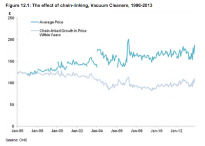
The process of chain-linking removes any price change caused by the products collected changing, as opposed to the prices of the products themselves changing. In other words, it shows the growth in price of the item as if there had been no change in the selection of products that make up that item. In terms of Figure 12.1, the difference in the two lines shows the increasing prices of the new products entering the basket, which can be seen as the quality of the products improving, over the 17 year period.
- Whilst the chain-linking in the CPI is undertaken in a slightly different manner and at different times, giving rise to double chain-linking, the effect is the same.
- The Johnson Review concludes:
Even though chain-linking is not referred to as a quality adjustment, in practice this is how much of the change in quality in items collected is accounted for in consumer price statistics. For example, in a new collection year, bread could be priced from a cheaper shop than in the year before. This reduces the average price of the products being collected, but there has been no change in the price of the products. The impact of this price change does not enter the price index, because of chain-linking.
Another example could be that in the future, 3D TVs might account for enough spending to be deemed representative of what households are buying. ONS could then broaden the description of TVs to include 3D TVs. This change will likely cause the average price for TVs to change, and this change will again be removed by chain-linking.
Chain-linking just aligns the price growth of different selections of products. It does not imply positive or negative quality change. It is therefore an implicit quality adjustment and does not control for any of the features, in terms of specification or location, of an item when there is a change in average price between years.
In practice, this means that goods and services whose quality is improving over time (such as technology goods) may show low or even negative rates of inflation, even though the typical price of a product of that type could be similar to what it was several years ago. It implicitly reflects quality change; the new products are more capable than the old ones.
- It is also important to consider the impact of a product or service becoming unavailable during the year, resulting in the need to select a replacement. This is a complex issue, the detail of which falls outside of the scope of this report, on which the ONS provides guidance as to how comparable replacements are to be selected. In the event that a new product is not considered to be suitably comparable with the previous product, the ONS has a range of tools that it can apply to ensure consistent comparisons over time.
- The Johnson Review sets out the following to illustrate the impact of the approach over time:
Figure 12.5 is identical to 12.1 but with the addition of a price index series for vacuum cleaners. This index is created using the Dutot formula (explained in Chapter 10). As in Figure 12.1, the difference between the top two lines shows the impact on average price of the quality of vacuum cleaners being collected changing between years.
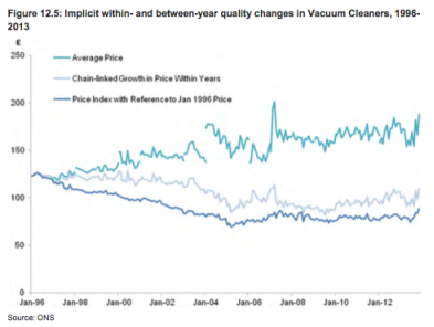
The price index controls for the effects of non-comparable replacements on average price, where as the middle line, chain-linked growth in price within years, does not. This means that if a product of higher price (and implicitly higher quality) is used as a replacement for another product it is treated as a price rise in the middle line, but is seen as a quality change in the index. The gap between the two lines can therefore be seen as the impact on average price of the quality of vacuum cleaners being collected changing within years.
Figure 12.5 shows a simplified example of the effect that discontinuation and replacement of products has on an index. Before 2004, the index falls compared with the middle line. This means the non-comparable replacement products are on average higher in price and quality than the original products. Between 2004 and 2008 however, the index is increasing at a faster rate than the middle line.
This implies that the replacement products are of a lower price over this period, and are implicitly of lower quality. However, for items with a short product life the choice of which products are comparable is very important.
- In terms of quality change over the long term, the Johnson Review states the following:
Over the long run, treating quality change appropriately poses additional challenges. Consider lighting, an example discussed by Nordhaus (1998). Over the course of hundreds of years, society has moved from candlelight to gas lamps to electric light bulbs. Each change in technology makes light cheaper. Over the same period, the cost of wax, then gas, and now electricity has been rising.
An inflation measure that puts a price on the means of making light (which is what the CPI does) would show a rise in prices. An inflation measure that puts a price on the cost of light itself would show a decline, because of the technological improvements over the same period. Astin (1998) makes a similar point about changes to the cost of listening to music over a period of 60 years. Indeed, Astin argues that the difficulty in comparing significant shifts in technology is such that consumer price indices are not ideal for making long-run comparisons over time.
This is an important issue but may simply reflect the limits of what a consumer price index can do. But it is something that people who use consumer price indices for very long term contracts, such as pension indexation, should perhaps consider.
- It is clear to the panel that neither of the primary consumer price indices available in the UK, the RPI and the CPI, is perfect, particularly over the long run. Specifically, the change in the value of the respective assumed baskets of goods and services is not a good match for the basket of goods and services that make up a personal injury claim and it is reasonable to assume that a claimant does not have the ability to substitute goods over time when compared with the average consumer (which accounts for much of the difference between the two measures). That said, it would be both impossible and impractical to have an adjusted discount rate for each element of the claim for the following reasons:
• Many elements of the claim will not have a suitable measure of their past cost, having removed qualitative improvements and/or the impact of general improvements in living standards; making it impossible to estimate how far out historical price changes for one element of the claim is outwith the RPI or CPI; and
• Even where there is such a historical measure of past differential, it is unlikely to be certain that any previous average of the differential will hold good annually over the claimant's future lifetime; and
• Even if such crystal ball gazing were considered appropriate, this would give rise to the application of so many discount rates in each and every case as to cause heightened conflict and complexity.
- Consequently, the panel understands that the inflation adjustment to the discount rate can remove speculation by reference to the yield on ILGS, but cannot remove the imprecision of applying a general measure of inflation, as distinct from the more precise path that periodical payments have followed.
- Both the CPI and the RPI meet the requirements of our brief with regards to the exclusion of the impact of general improvements in living standards and qualitative improvements, insofar as steps are taken to remove any such impact.
- Clearly, ILGS are linked to changes in the Retail Price s Index (all items); the RPI. The RPI is acknowledged by the Office for National Statistics as being flawed; in March 2013 the RPI was downgraded from being a "National Statistic", and might now fail the test of a reliable measure established by Mackay J in RH[2], for the following reasons:
1.2.1 The Statistics Authority judges that the RPI, including the sub-indices and variants listed in section 1.1.2, does not comply with Principle 4 and specifically with Principle 4, Practice 5 of the Code. This view is based primarily on:
- the finding that the methods used to produce the RPI are not consistent with internationally recognised best practices (para 3.4); and
- the decision to freeze the methods used to produce the RPI, and only to contemplate routine' changes (para 3.5).
- As a result, many pension schemes and State benefits have already switched to the government's preferred measure of inflation, the CPI, and the future issue of CPI- linked gilts would not be surprising. Furthermore, guaranteed income payments under the no-fault statutory compensation scheme for members of the armed forces injured in service are also linked to the CPI.
- There is also evidence of an increasing wedge' between CPI and RPI. Historically, CPI has been around 0.7% pa below RPI. However, in its paper of November 2011 entitled "The long-run difference between RPI and CPI inflation" the Office for Budget Responsibility (OBR) states that it expects the wedge' to rise to between 1.3% and 1.5% pa. Importantly though, the OBR set out the following in their March 2015 "Economic and fiscal outlook":
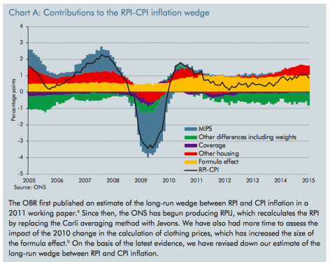
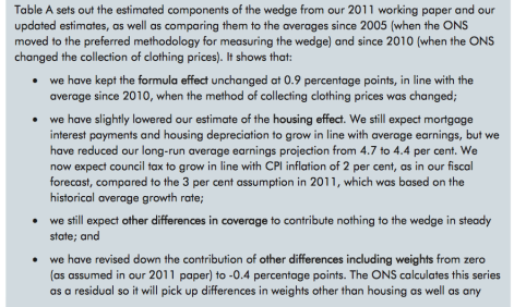
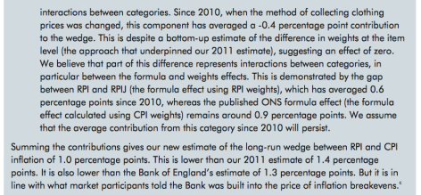
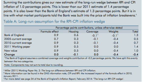
- It is clear from the above that the largest contributor to the difference between the two inflation measures is the formula effect'.
- According to the OBR, the geometric mean is "better suited to accounting for the effect of substitution between goods and services when relative prices change. The [geometric mean] of a given set of non-identical positive numbers is lower than the [arithmetic mean] of the same set of numbers."
- The CPI is held to be the more accurate measure of price inflation in the UK economy and, therefore, preferred by the government. Indeed the Johnson Review concluded:
The Authority and ONS should make it clear to users that the RPI is not a credible measure of consumer price change. The RPI should not be used for new contracts. Taxes, benefits and regulated prices should not be linked to the RPI.
The RPI should also not be used as the measure of inflation when comparing living standards over time, at least for recent years where better consumer price indices are available. The issuance of index-linked gilts is more complex, but government should move away from selling gilts linked to the RPI, subject to consultation and assurance about the demand for CPI or CPIH linked gilts.
As the headline RPI is not a robust measure of inflation, it makes little sense to continue to produce analytical indices, such as the Pensioner Price Indices and the Tax and Price Index, which are based on the RPI. Where there is demand for analyses of this type to continue, these can be replicated on a CPIH basis (where they are not already), or within the scope of the subgroups analysis set out in recommendation 2.
- Unlike linking a new PPO to the RPI, relying on the RPI for the basis of the discount rate is not, in our eyes, a new contract, but a reliance on existing contracts for RPI- linked ILGS. That said, on the basis of the above it is clear that on current long-term forecasts the RPI is positively biased, as a measure of price inflation compared to the CPI, by around 1% per annum.
- Actuaries make assumptions about RPI and CPI levels when valuing pension scheme liabilities and a recent survey of IAS19 Assumptions suggested that RPI might be expected to outpace CPI by 0.95% p.a. [1]
- As a result, it is appropriate to address whether the RPI-based yields considered in Chapter 1 should be upwardly adjusted to take this wedge into account. We consider that there is some difficulty in doing so, as we are of the view that claimants are unlikely to be able to substitute needs in the same way as the average consumer (with the assumption in respect of substitution accounting for the majority of the wedge) and, particularly, given the contents of Table A above. Whilst these are stated as being long-term' estimates, it is our understanding that they would not be considered robust over a 40 to 60-year duration; which is the duration of loss in many personal injury cases.
- To illustrate the difficulty, if the discount rate had been increased by 1.4% following publication of the OBR estimate of the long-run wedge in 2011, the fact that the wedge has been 0.7% means that significant under-compensation would have occurred.
- That said, we refer back to our primary instructions which state that:
The discount rate relates to the real rate of return[2] that the market will provide to the claimant as a reward for forgoing the use of the capital he or she invests.
- In this regard we note that the Bank of England is the market maker in respect of RPI- linked gilts and continues to issue them through the Debt Management Office (DMO). However, market yield on any gilt can only be derived from observation of actual trades (as distinct from the yield at issue), and there is no market in CPI-linked gilts. In other words, there is no market rate to refer to in making an adjustment for the wedge.
- The Johnson Review states the following with regards to the issuance of RPI-linked gilts:
The RPI is still used in large numbers of commercial contracts, including in £470 billion worth of index linked gilts. The sale of these gilts is used by the government to fund part of the national budget deficit. Some of these gilts will not be redeemed until 2068 and in future new gilts may be issued with even longer terms. And the continued existence of long-term liabilities linked to the RPI continues to create demand for assets that provide returns also linked to the RPI, regardless of the statistical issues.
So despite its statistical inadequacy, the RPI cannot simply be discontinued. Indeed, cognisant of these needs, ONS also noted that there is significant value to users in maintaining the continuity of the existing RPI's long time series without major change' (ONS, 2013). It was with this in mind that the National Statistician recommended that the formulae used at the elementary aggregate level in the RPI should remain unchanged.
The UK Statistics Authority and ONS have important roles to play in communicating the primacy of CPIH, explaining what it is measuring and how it should be used. The Authority and ONS should also be very clear in explaining that the RPI is not a credible measure of consumer price change. They should make it clear that the RPI is not fit for purpose and should not be used except where existing legal contracts – for example index-linked gilts – demand it. If a way can be found to discontinue the production of the RPI while maintaining the integrity of these legal contracts then it should be pursued. In the course of the review we have not found a satisfactory solution to this conundrum.
The UK Statistics Authority has a duty in UK law to produce the RPI (Statistics and Registration Service Act 2007, Section 21). Some of the current uses of the RPI will be very hard to unpick. For example, index-linked gilts currently link to the RPI. Some of the index-linked gilts currently in issue will mature as late as 2068. Some gilts allow the holder to redeem the gilt in the event of a fundamental and detrimental' change to the RPI. The last of these mature in 2030. Many other statutory and contractual uses of the RPI will be difficult, and potentially costly, to change. It seems impossible to discontinue the RPI in the short term.
- To adjust the discount rate for any specific rate of assumed long-run positive bias in the RPI over the CPI seeks to add a level of precision and a degree of uncertainty that is outwith the rest of the theoretical calculation adopted in Wells, as all of the other elements remove the need to attempt to forecast the future. This conclusion is consistent with our view set out above that it is inappropriate to adjust the discount rate for a specific personal rate of inflation applicable to the basket of goods and services in a particular case.
- In the event that CPI-linked ILGS are released by the Bank of England, assuming that they are in sufficient number and duration, it is our view that this would be a potential trigger for the reconsideration of the discount rate.
- With regards to any adjustment for real growth in heads of claim relative to RPI, it is our view that no such adjustment can be made given the contents of our instructions for the task. The panel agrees that any long-term real growth in the price of goods and services is driven by either:
• Qualitative improvements; and/or
• Productivity improvements; and/or
• General improvements in living standards.
- In respect of future care and case management, often the largest and most important element of a claimant's award, the inclusion of pay-drift' was fully considered in all of the Thompstone et al first instance cases and at the Court of Appeal. As noted above, the fact that a Periodical Payments Order can embrace real growth in the price of future care and case management does not foul Cookson -v- Knowles, as the measure being applied to uprate the annual payments is neither being applied to a multiplicand or multiplier. It is not a matter for the panel to consider the continuing suitability of the principles established in Cookson -v- Knowles.
- It is the majority view of the panel that there would be a fundamental inconsistency with the principles set out above if the discount rate was to be set by embracing an investment portfolio including real (risk) assets, the returns on which would be expected to reflect general improvements in the standard of living.
- In conclusion, the panel consider that the discount rate should be adjusted for inflation as measured by the RPI, the basis of indexation of ILGS. Given the constraints on the parameters of our advice, no adjustment should be made to the discount rate for any differential between the increase in the price of goods and services within a claimant's claim when compared to the RPI or the wedge between RPI and CPI, nor can any adjustment be made in respect of real earnings growth or real price inflation of any specific good or service that the claimant will need to purchase in the future.
A financial economics approach to the discount rate Summary
- This chapter adopts a financial economics approach to the discount rate. In adopting this methodology it is implicitly assumed that a departure from a risk-free/market consistent approach, as considered in Chapters 1 and 2, is still consistent with the principles adopted in Wells and by the Lord Chancellor in 2001.
- This is a minority view of the panel. The majority of the panel are not persuaded that this is correct, but ultimately it is a matter for the Lord Chancellor to decide.
- A financial economics approach can arrive at a range of discount rates, depending on appetite for non risk-free assets. The panel has alighted on two portfolios within a range that might be deemed appropriate.
- The first is a combined portfolio that has one-half invested in ILGS and one-half in the optimal mix of risky investments. This has only half the investment risk than if the whole amount was invested in the optimal risky investment portfolio.
- Based on the analysis contained in Appendix 2, the emerging discount rate is 0.75% and the risk (standard deviation) +/- 2.5%.
- The majority among the panel do not believe that this portfolio is potentially appropriate for a very low risk, but not a risk free', investor and the 100% rule. The minority view is that this portfolio would be appropriate. If adopted, it would be a matter for the Lord Chancellor to decide whether to round the rate up or down, to the nearest one-half of one per cent.
- The second is a combined portfolio that has three-quarters invested in ILGS and one- quarter in an optimal mix of risky investments. This has only one-quarter the
investment risk than if the whole amount was invested only in the optimal risky investment portfolio.
- Based on the analysis contained in Appendix 2[1], the emerging discount rate is 0% and the risk (standard deviation) +/-1.25%.
- The panel is in complete agreement that, if forced to accept some investment risk, then the second portfolio (three-quarters ILGS and one-quarter in an optimal mix of risky investments) is potentially appropriate for a very low risk, but not a risk free', investor and the 100% rule.
- The panel is also in complete agreement that portfolios combined using less than one- half invested in ILGS and more than one-half invested in the optimal mix of risky investments are inappropriate for a very low risk investor – the risk is too high. Further detail on the material discussed in this chapter is provided in Appendix 2.
- Case law, and the basis of our instructions, indicates that the hypothetical claimant in a personal injury situation must be regarded as having very low risk tolerance. A very low risk tolerant investor may at least be expected to assume some investment risk, and if the pool of potential investments is extended beyond risk free investments then this makes a financial economics approach, rather than the risk-free market consistent approach considered in Chapter 1, a possible alternative way to establish the discount rate.
- A financial economics approach uses the long-run rate of return on an investment portfolio to determine the discount rate. Actuaries use risk-free discount rates in very many insurance and pension applications, as discussed in Chapter 2, but in other applications, say when ongoing contributions are being made to a pension fund with an excess of assets over liabilities and a sponsoring employer with a strong covenant,
discount rates could be set with reference to non-risk-free benchmarks.
- The financial economics approach to setting the discount rate in a personal injury context is to use the long-run rate of return on a very low risk investment portfolio. Appropriate investment metrics and measures need to be applied to establish that the investment portfolio is very low risk. No single investment metric is sufficient to do this and a combination is needed. Once a very low risk mixed investment portfolio has been determined, the discount rate is the long run real expected return on the portfolio, after taxation and management expenses.
- Downside risk measures are the most important for this study because the claimant is assumed to draw a regular income from the portfolio. If the portfolio falls relative to RPI, more units of the fund have to be encashed than intended to pay the same real income to the claimant. If the fall relative to RPI is persistent more units will again need to be encashed. The effect will be similar if the fall is short but substantial. In both cases, a higher long-run future investment return may then be required in order to be able to sustain the same regular income into the future, and that may not be achievable while maintaining very low investment risk.
- The type of risk described above is called sequencing risk, and is critically important when drawing an income over time from an investment portfolio. Sequencing risk occurs where one year of below RPI investment returns is immediately followed by another, which is immediately followed by another etc. Poor investment return sequences combine with portfolio withdrawals in a highly destructive way because more fund units need to be enchased to generate the same annual income. The double erosion of capital following a market fall - the market drop and the drawing an equal income at depressed fund value - is what makes sequencing risk potentially destructive. One of the lessons of the technology boom and bust followed shortly by
the financial crisis was the importance of the order, or sequence, of extreme investment returns. If a sequence of market drops means the capital of a fund is 50% lower than planned, a 100% gain is needed to return the fund to where it should be. By knowing about sequencing risk portfolios can be constructed to reduce it.
- Standardised general measures of variability, of which standard deviation is by far the most used, are less important in an income drawdown environment, but standard deviation remains very useful when it comes to making statements about likelihood and attaching a level of confidence to a particular set of results reoccurring. If the investment portfolio constructed has approximately normally distributed investment returns, more informed statements about likelihood and chance can be made.
- Chapters 1 and 2 considered the issue of setting the discount rate by reference to risk free returns, in excess of the RPI, as discussed in Chapter 3. A set of risk free investments is envisaged, matching the anticipated cash flows as they fall due in future. A portfolio of ILGS is envisaged. This chapter takes a financial economics, mark-to-market, fair value, total return approach. A mix of risky investments is assumed to be held, increasing return. There will as a consequence be variability around the short-term, mark-to-market value of the portfolio, but as long as this is deemed to be tolerably small such portfolios may, for some investors who can tolerate risk, fit with a very low risk investment approach.
- To construct a potentially appropriate mixed investment portfolio, two long-run datasets are used that industry and academia hold in high regard. These are the Barclays Equity Gilt study and the Dimson, Marsh, Staunton, datasets. Both are based on annual investment performance data from 1900 to 2014 inclusive, to give 115 years of data. This time period includes deflation and inflation, the two World Wars, and since 1980 the dotcom boom, bust, financial crisis, US crash of 1987, 1997 Asian foreign exchange crisis, as well as different economic regimes – RPI from 9% to 1%, recession and boom.
- The asset classes need be to be diversified and so should be held in the form of index investments. Fund managers establish low charge funds for investors that replicate these indices. There will be transaction costs involved in managing the investments, as well as management costs and charges. To allow for this the analysis deducts 100 basis points, or 1%, from the annual performance of each bond index as an estimate of the after cost performance and 1.25% annually from each equity index. This includes an allowance for tax [1]. All the figures quoted throughout this report are after deducting these amounts – i.e. all figures are net of costs, charges and taxes. We appreciate that this is a broad brush' approach to the question of the appropriate deductions for tax and management expenses, which is open to challenge, but time constraints have not permitted a fuller investigation of this issue.
- The following five downside risk measures are used to determine whether an investment portfolio is very low risk:
• Sequencing risk.
• Drawdown.
• Downside deviation.
• Value at Risk.
• Conditional Value at Risk.
These five risk measures must point to a very low likelihood of distressed selling and strong protection of capital relative to RPI. To be consistent with the investment risk objective the portfolio assembled will need to have:
• Very little sequencing risk i.e. not be prone to a succession of below inflation investment returns.
• Very limited peak to trough drops in market value (drawdown risk).
• A low level of downside risk (semi-variance, downside deviation, and Value at Risk).
• Low exposure to tail risks within the worst 5% of expected investment returns (Conditional Value at Risk).
• A narrow dispersion of real returns over time (tracking error to RPI, standard deviation).
- We consider these to be the key metrics to judge suitability when taking a financial economics approach. These metrics are more fully described in Appendix 2.
- An optimal investment portfolio is identified using a technique developed by financial economists known as modern portfolio theory. This combines assets in an optimal way, assigning more weight to assets having low correlations with one another. The requirement to adopt modern portfolio theory is embedded within prudent investor rules and the concept of fiduciary duty both in the UK and overseas. The analysis at Appendix 2 concludes that the optimal mix of risky investments is 50% in corporate bonds, 30% in overseas developed country government inflation linked bonds, and 20% in equities.
- The panel is in complete agreement that the risk measures associated with this optimal mix of risky investments is too high. The expected annual real investment return is 2.5%, significantly above risk free returns, with standard deviation (risk) of +/-5.0%.
- A way of reducing risk is to only invest one part of the investor's capital into the optimal mix of risky investments and the other part in risk free investments (ILGS). Two portfolios have been analysed that could, for some investors, be considered to be
very low risk. The two portfolios chosen are based on the same optimal mix of risky investments. The two portfolios differ only by the proportion held in the optimal mix of risky investments and the proportion held in risk free investments. We are conscious that if departing from a risk free investment approach that very low risk' is something that will mean different things to different investors. There is not a unique answer to the problem, once a departure is made from a risk free framework.
- The two portfolios have been relatively stable through different market regimes. Neither portfolio has significant sequencing risk, and both have approximately normally distributed investment returns.
- The first of the two portfolios has 50% of the investments in ILGS (presumed to have no risk), 25% in corporate bonds, 15% in overseas developed country government inflation linked bonds, and 10% in equities. The expected long-run annual real investment return on this first portfolio is:
Asset | Portfolio weight (%) | Portfolio return (%) |
Risk free/ILGS | 50 | -1.0% [1] |
Corporate bonds (25%), Overseas developed country government inflation linked bonds (15%), Equities (10%) | 50 | 2.50% |
The expected investment return is (50% x -1.0%) + (50% x 2.5%) = 0.75%.
4.27 This first portfolio has a standard deviation of real investment returns of 2.5%. The standard deviation tells us that over time[2]:
• Two in every three years the real annual investment return is expected to be between -1.75% and 3.25% from RPI.
• Nineteen in every twenty years the real annual investment return is expected to be between -4.25% and 5.75% from RPI.
4.28 The second portfolio has 75% of the investments in ILGS (presumed to have no risk), 12.5% in corporate bonds, 7.5% in overseas developed country government inflation linked bonds, and 5% in equities. The expected long-run annual real investment return on this second portfolio is:
Asset | Portfolio weight (%) | Portfolio return (%) |
Risk free/ILGS | 75 | -1.0% [3] |
Corporate bonds (12.5%), Overseas developed country government inflation linked bonds (7.5%), Equities (5%) | 25 | 2.50% |
The expected investment return is (75% x -1.0%) + (25% x 2.5%) = -0.125%,
rounded to 0%.
- This second portfolio has a standard deviation of real investment returns of 1.25%. The standard deviation tells us that over time:
• Two in every three years the real annual investment return is expected to be between -1.25% and 1.25% from RPI.
• Nineteen in every twenty years the real annual investment return is expected to be between -2.5% and 2.5% from RPI.
- The panel has mixed views, as set out above, about the appropriateness of the two portfolios, and, on the matter of the reasonableness of departing from a risk-free framework.
- It is a matter for the Lord Chancellor to consider whether such a departure is appropriate.
Should Discount Rates Vary by Duration of Loss?
- A further consideration is whether the discount rate should vary by term of loss. This is an issue that has been considered by the Courts in Canada, where the Province of Ontario prescribes a different market related risk free rate to apply to damages of terms up to 15 years, being 0.3% in 2015 (it changes each year), with a higher fixed discount rate of 2.5% applying for longer durations. [1] The Courts in Hong Kong have adopted a different approach, but still acknowledging the presence of a term structure' for discount rates with the discount rate being -0.5% for terms of loss not exceeding 5 years, 1% for terms not exceeding 10 years and 2.5% for terms exceeding 10 years [2].
- This use of discount rates that vary by term has its attractions on theoretical grounds. Chapter 2, which discussed how actuaries calculate and use discount rates in more general applications, raised the point that insurers reserving for long term liabilities use discount rates which, subject to technical adjustments beyond the scope of this discussion, are the nominal risk free rates for each term of valuation of a liability cash flow. The level of inflation assumed in the underlying cash flow is a separate consideration. A different discount rate is then in fact used for each future year. For the Courts, and the legal profession, dealing with volumes of cases over many years such complexity would be highly undesirable.
- We consider a number of issues to be relevant in this regard:-.
• If the discount rate, net of inflation in the head of claim, taxation and management expenses is set with regard to ILGS alone, the issue of term structure is less relevant.
• The claimant is assumed to purchase all of his ILGS at the point of settlement, so can only invest and secure the yield which is available at the time of receipt of his award of damages. To the extent that higher (or lower) yields may be available in future is of relevance only in the re-investment of income, and a claimant is expected to expend income (and capital) annually over the expected period of loss. The initial available levels of investment yield are then of primary importance.
• Considering the yields in the ILGS market the yield curve currently is extremely flat for longer durations as shown in the table below:
Real Yield (above
Term RPI)
<5 -0.7%
5 to 15 -0.7%
>15 -0.9%
• There is similar evidence of a flat term structure in the yields available on conventional (non-index linked) securities. Here the nominal yield can be thought of as the risk free yield plus implied RPI inflation, possibly subject to a risk premium.
Nominal Term Yield
5 1.7% 10 1.9% 25 2.4% 50 2.5%
• As considered earlier, the ILGS market extends to c50 years, when the maximum period of loss for a personal injury claimant could extend to c90 years. The ILGS market then gives us no guidance to the level of risk free real yields beyond 50 years, although the very flat term structure between 10 and 50 years suggests that yields beyond 50 years may differ from those for durations under 50 years only to a quite modest extent. In a practical setting a claimant can only invest in 50-year gilts and take his or her chances on the level of re-investment yields at this future time. Future yields are then important for such a class of claimants. That said, for the majority of claimants, the duration of the ILGS market extends beyond the expected period of loss.
• As discussed in earlier chapters, the actuarial profession considers the issue of discount rates (on a market consistent basis) beyond durations available in the market for government debt. As an example, the nominal discount rate for a liability in 50 years is 2.1% but the nominal discount rate for a liability in 90 years is 2.8%. We are, of course, interested in the discount rate net of inflation in the head of claim. Little research material is available which considers this issue but parameters used in the modelling process by EIOPA show that, when considering ultimate forward rates', risk free rates are around 50% of assumed nominal returns. This would suggest that, if setting a discount rate for the broadest category of cases, including those of the very longest terms of loss, one might be inclined to use a discount rate for these longer terms, say, 0.4% higher than those for terms used for 50 years.
• On the assumption that the discount rate continues to be set by consideration of ILGS yields then there is some justification for using a modestly higher discount rate that might be obtained solely by inspection of yields available up to 50 years in duration. The impact of any allowance however seems likely to be modest and we would therefore support use of a discount rate which does not vary by the duration of loss.
• Chapter 4 considered possible levels of the discount rate if it were felt that a mixture of ILGS and an optimally constructed portfolio of risky' investments were still felt to be consistent with the principles of Wells. The concept of a term structure for discount rates does not extend naturally to non-risk free investments but some consideration might conceivably be given to valuation frameworks incorporating risk free discount rates, of say -1%, at short and medium duration with mixed portfolio' discount rates of, say 0% or 0.5%, at the longest durations.
Summary and Recommendations
- We have reviewed the historic background to the setting of the discount rate and carefully considered the directions given by Counsel for the MoJ on the constraints within which our advice has to be provided.
- Findings and recommendations are summarised below according to the following
three categories:
- General agreement among all the panel.
- Some agreement among the majority of the panel, although not necessarily all the panel.
- Mixed views where the panel members hold mixed opinions and the view of a minority of the panel is being expressed.
General Agreement
- A reworking of the analysis performed by the Lord Chancellor in 2001 would suggest an appropriate discount rate, were it to be assessed through a consideration of ILGS yields, would be -1%, rounded to the nearest half of one per cent.
- The panel all agree that the problem faced by the Courts, when assessing the lump sum award to provide for future losses or costs, can be considered to be an essentially actuarial problem. We have therefore reviewed actuarial practice in the setting of discount rates more generally. Actuaries support use of a market consistent approach to the setting of discount rates when dealing with valuations of future cash flows for
transactional or reserving purposes. An award of damages is a transaction from the perspective of the defendant and provides a reserve for claimants to provide for future losses as they fall due. Risk free discount rates should then be used in the valuation exercise. Insurance examples are considered (e.g. Solvency II) and it is noted that risk free rates are used to value liabilities irrespective of the nature of the underlying assets being held as reserves for the liability cash flows. Surveys of discount rate assumptions used by insurers when reserving for periodical payments ("PPO") liabilities demonstrate that insurers use risk free discount rates, which vary depending on assumptions they make regarding the movement of PPO indexation variables relative to the RPI (being the basis of indexation of ILGS). Actuarial practice is supportive of the use of risk free discount rates in the context of quantifying an award of damages. ILGS provide a measure of these risk free rates.
- ILGS provide a guaranteed return relative to the RPI but it is not clear that the RPI is necessarily reflective of inflation' in a broader sense. The RPI tends to outpace the CPI, but neither can be assumed to necessarily be representative of the likely level of inflation in various heads of claim. Some of these might be earnings related, some might not. We have been instructed to assume that productivity related elements of inflation are to be disregarded (e.g. real earnings growth). On balance we are supportive of the view that the RPI is an acceptable measure of inflation to use when setting the discount rate. ILGS conveniently provide a directly observable measure of yields relative to RPI. Yields relative to other measures of inflation, CPI, ASHE indices, etc. can only be estimated, they are not observable.
- Only ILGS/risk free investments can provide a certainty of returns relative to RPI, and
a predictable level of return relative to other forms of inflation. They are an optimal fit
to the view of the Courts that there can be no question about the availability of the money when the investor requires repayment of capital and there being no question of loss due to inflation'. One might call this the notional annuity approach'.
- We are not persuaded that the discount rate needs to vary by term of loss at the current time, if the discount rate is set by reference to ILGS alone, as the real interest rate yield curve is relatively flat over long durations. This may change as market conditions alter and should be kept under review.
- The panel is however tasked with considering the risks and returns from other categories of investments and combinations of these investments.
- Dr Cox has extensively analysed historic returns (net of estimated reductions for taxation and management expenses) from categories of investments potentially available to claimants investing an award of damages. Using modern portfolio theory techniques it has been possible to construct what one might describe as the optimal' portfolio offering a balance between return and risk. Dr Cox then considered a range of potential measures of risk for the selected portfolio, with specific attention being paid to downside' measures of risk. Having reviewed the research the panel is of the opinion that the emerging risk measures are inconsistent with the requirement for the portfolio to be considered very low risk'. The panel is in agreement that the investment risk of 100% in the "best risk portfolio" is too high. This is covered in detail in Chapter 4 and Appendix 2.
Some Agreement
- It is the minority view of the panel that the problem faced by the Courts, when assessing the lump sum award to provide for future losses or costs, can be considered using a financial economics approach.
- The level of risk is too high when 100% is put into the optimally constructed portfolio of risky assets but the risk can be moderated by combining the chosen portfolio with real risk free investments. The lower the proportion of risky investments the lower the risk, and the lower the return. In order to provide very low' levels of risk there is some agreement among the panel that up to 25% of the portfolio could be allocated to non-risk free assets. In such circumstances the discount rate would be 0%.
Mixed Views
- A minority among the panel believe that slightly more than 25% but no more than 50% of the portfolio could be allocated to non-risk free assets. If 50% was allocated to non-risk free assets, the discount rate would be 0.75%.
- The illustration overleaf brings together the discount rates the panel have alighted upon using the risk-free/market consistent and financial economics techniques discussed more fully in Chapters 1 and 4 respectively, as well as illustrating the corresponding level of panel agreement.
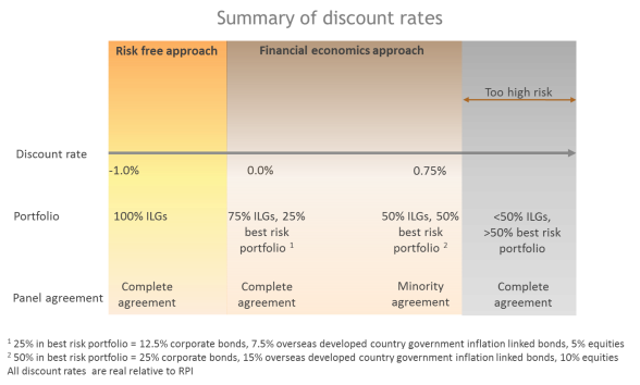
- The panel are hopeful that this report is of some assistance to the Ministry of Justice and we would be pleased, collectively or individually, to discuss matters in due course. Ultimately it would appear that the Lord Chancellor's decision is one of whether a very low risk' portfolio or a risk free' portfolio is consistent with the current legal framework. What is clear to the panel is that the current discount rate of 2.5% is inconsistent with current market conditions, with a risk free approach suggesting a discount rate of -1% and a very low risk' mixed portfolio approach suggesting a discount rate of 0% to 0.75%.
Sources of data and evidence used
A1.1 Data sources are acknowledged within the report as a whole. In addition, the panel
has considered the following:
• Responses to the first consultation paper ("DR1") issued by the MOJ in 2012.
• IPSOS Mori personal injury discount rate research published in 2013.
Responses to DR1
A1.2 There were 63 individual written responses to DR1, and a small number of ad hoc
responses by email. Respondents were self-selecting: this is not an independently drawn sample.
A1.3 Not all of the written responses were in the form of the DR1 questionnaire. Some
respondents chose only to deal with specific questions, or made general observations.
A1.4 Only four of the DR1 questions could be answered with a simple yes or no: these
questions, and the responses to them are summarised in the table overleaf. For the purposes of presenting the evidence, respondents who submitted the questionnaire have been allocated to the following groups, so as to reveal any particular bias or strength of opinion:
- Professional bodies and the judiciary.
- Organisations or firms particularly associated with claimants.
- Organisations or firms particularly associated with defendants.
- Individuals not particularly associated with claimants or defendants.
A1.5 Unsurprisingly, these groupings reveal a polarisation of views between the respective
interests, economic or otherwise, in the outcome of the Lord Chancellor's review of the discount rate.
Do you agree that setting
Should any allowance be the discount rate on the
Do you agree that the
made for potential basis of expected returns Do you agree that one claimant should be
differences between RPI from a mixed portfolio of prescribed discount rate assumed to hold all
inflation and health care assets is consistent with is sufficient? ILGS until redemption?
costs inflation? the House of Lords
decision in Wells v Wells?
Council of HM Circuit Judges Yes Yes No Yes Faculty of Advocates Yes Yes Yes No Law Society of Scotland Yes Yes No No Liverpool Law Society Yes Yes No No Ogden Working Party (dissenting views) No Yes Yes No Ogden Working Party (majority response) Yes Yes No No Senators of the College of Justice Yes Yes No No The Personal Injury Bar Association Yes Yes No No
![]() Yes 88% 100% 25% 13% No 13% 0% 75% 88%
Yes 88% 100% 25% 13% No 13% 0% 75% 88%
Association of Personal Injury Lawyers Yes Yes No No AvMA (charity) Yes Yes No No Forum of Complex Injury Solicitors Yes Yes No No Motor Accident Solicitors Society Yes Yes No No Mr Grahame Codd, Irwin Mitchell LLP (Solicitors) & Mr Ed
Tomlinson, IM Asset Management (investment managers) Yes Yes No No
Mr Julian Chamberlayne, Stewarts LLP (Solicitors) Yes Yes No No Mr Paul Kitson, Slater & Gordon (UK) LLP (Solicitors) Yes Yes No No
![]() Yes 100% 100%
Yes 100% 100%
No 100% 100%
Admiral Group Insurance Ltd (insurer) No No Yes Yes Ageas Insurance Ltd (insurer) No No Yes Yes Allianz Insurance Plc (insurer) No No Yes Yes Aviva (insurer) No No Yes Yes AXA (insurer) No No Yes Yes eSure Insurance Ltd (insurer) No No Yes Yes Forum of Insurance Lawyers No No Yes Yes Groupama Insurances (insurer) No No Yes Yes Kennedys (Solicitors) Yes No No Yes Lloyd's Market Association No No Yes Yes Medical and Dental Defence Union of Scotland No Yes Yes No Medical Defence Union No No Yes Yes Motor Insurers' Bureau No No Yes Yes Mr Adrian Dagnall, Bevan Brittan LLP (Solicitors) No Yes Yes Mr Douglas Russell, Simpson & Marwick (Solicitors) Yes Yes Mr Geoff Owen, Greenwoods (Solicitors) No No No Yes Mr Andrew Ireland, Law Society of Scotland, personal response No No No Yes Mr Mark Bailey, Morgan Cole (Solicitors) No No Yes Yes Mr Michael McKenna & Mr David Locke, Hill Dickinson
(solicitors) No Yes Yes Yes
Mr Stephen Dewar, Munich RE (Reinsurer) Yes No Yes Yes NFU Mutual (insurer) No No Yes Yes NHS Litigation Authority Yes No No Yes QBE European Operations (insurer) No No Yes Yes RSA (insurer) No No Yes Yes Swiss Re (reinsurer) No No Yes Yes Zurich Insurance plc (insurer) No No Yes Yes
![]() Yes 13% 12% 85% 96% No 88% 88% 15% 4%
Yes 13% 12% 85% 96% No 88% 88% 15% 4%
Charles Stanley & Co Ltd (investment managers) No Yes Yes Yes Frenkel Topping (independent financial advisers) No Yes Yes Yes Grant Thornton LLP (accountants) No No Yes No Mr Andradvisers) ew Sands, Nestor Partnership LLP (independent financial Yes Yes No No
Mr Chris Daykin (actuary) Yes Yes No No Mr Maurice Faull, Hilton Sharpe & Clarke (accountants) Yes No No Yes Mr Paul Meins (actuary) Yes No No Yes Mr Richard Cropper & Mr Ian Gunn, Personal Financial Planning
Ltd (independent financial advisers) Yes Yes No No Mr Rowland Hogg (accountant) Yes Yes No No
![]() Yes 67% 67% 33% 44% No 33% 33% 67% 56%
Yes 67% 67% 33% 44% No 33% 33% 67% 56%
Rounding means that in some cases the total yes/no responses shown do not equal 100% The groupings shown are for illustrative purposes only to indicate views at a general level
IPSOS Mori Personal Injury Discount Rate Research
A1.6 In total only 14 people were involved in this research, which is caveated accordingly, i.e. that the findings cannot be generalised to the wider population, and that the very
small sample size of claimants has no statistical significance. The qualitative research deals with what is actually done with an award of damages. This has no bearing upon
the process of setting the discount rate.
A1.7 The quantitative research showed there were 766,417 personal injury settlements in
2011/12. There was no breakdown of the settlements. The extent to which they included damages for future loss, and were affected by the discount rate, is unknown. However, unsurprisingly, the research also highlights the sensitivity of claims that are affected to a change in the discount rate.
A1.8 Using qualitative data, the researchers estimated that only around 10% of settlements
include damages for future loss, which would typically represent 70% to 90% of a lump sum settlement. Whilst more than half of road traffic accident claims involved males aged under 30, the research was inconclusive as to whether this group is more likely to be affected by the discount rate.
A1.9 Qualitative research confirmed that, behaviourally, claimants tend to behave as might
be expected when making financial decisions about the investment of an award of damages, i.e. they exhibited caution when making investments, and risk-aversion.
A financial economics approach to the discount rate – an expanded discussion.
Section A: Holdings of UK ILGS by pension funds and life insurers
Introduction
A.1 This appendix adopts a financial economics approach to the discount rate. A very low
risk mixed investment portfolio is constructed and the long-run expected investment return used as a discount rate consistent for a very low risk investor.
This first section examines industry practice to develop an understanding of the investment allocation to ILGS and other assets by pension funds and life insurers who have long term inflation linked liabilities exceeding £1.5 trillion. This section finds that many UK financial institutions with contractual obligations to make future inflation linked payments to members do not only hold ILGS. Given the size of the ILGS market relative to insurer and pension liabilities this is not especially surprising, and, as was discussed in Chapter 2, the investments made by insurers and pension funds are not necessarily relevant to the setting of the discount rates used to value their corresponding liabilities.
A.2 The chart below shows cumulative net purchases of ILGS (in billions) by pension funds and insurers in UK index-linked gilts (green line) and a measure of the per cent
held of the UK ILGS market (blue line). The blue line is calculated as cumulative net purchases (green line) divided by the cumulative issuance of long-term index-linked gilts[1]. The left panel reports pension funds and the right panel life insurers. The
starting value of the green line is the stock of ILGS held as of Q1 1987. The starting value of the blue line is the market value of the stock of ILGS held by these financial institutions divided by the market value of long-term ILGS as of Q1 1987.
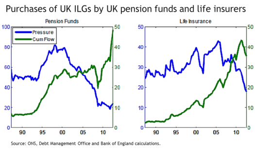
A.3 The per cent of the ILGS market held by pension funds reached a peak around 1998,
with the introduction of the minimum funding requirement in the Pensions Act 1997. The per cent of the ILGS market held by life insurers also increased around regulatory changes in 1997 and 2004. From year 2000 for pension funds and year 2008 for life insurers, relative holdings of the ILGS market have been falling, and pension funds and life insurers together now hold around 40% of ILGS issuance. The key takeaway from this chart is that financial institutions continue to invest in ILGS, but purchases are not keeping pace with issuance, so the per cent held of ILGS in issue has been falling. This evidence disconfirms the hypothesis that demand pressure from pension funds and insurers is partially responsible for pushing up the price of ILGS and driving down ILGS yields to artificially low levels. As was discussed in Chapter 1, the downwards trends in yields available on inflation protected securities has in fact been part of a worldwide phenomenon, associated with declines in real economic
activity in recent years and an increased focus on saving at the expense of consumption.
The ILGS Yield
A.4 The investigations above suggest that ILGS are unlikely to be the only asset in the
portfolio of investors with long-term inflation linked liabilities.
A.5 ILGS are held for risk management reasons or as a diversifier in a wider portfolio
context, but low or negative real yields are making further holdings of ILGS a real challenge for many trustees and investment officers.
A.6 There has been a growing trend over the past 15 years for pension funds and insurers
with large annuity businesses to hold other assets. These other assets are held to generate higher returns.
A.7 The chart below presents UK annuity writers' (i.e. life insurers) average asset
allocation. Note the large proportion of corporate bonds held (left panel). Note also that within the corporate bond allocation there are significant holdings of low quality corporate bonds (right panel), where expected returns are higher still. Holdings of government bonds have not increased with total assets, leading to the declining proportion held, as noted in the previous chart.
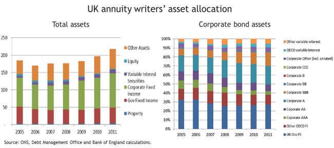
A.8 Pension funds' overall asset allocation over the same time period, shown below,
differs primarily by their higher holdings of UK and overseas equities. Equities help to hedge the inflation risk in their liability cash flows and to earn additional return
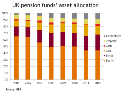
A.9 The takeaways from this first section are as follows:
- ILGS represent the closest there is to a risk free asset and are a risk free benchmark that any portfolio should be measured against, but that doesn't necessarily make ILGS the appropriate or optimal investment strategy for an investor who can tolerate a degree of investment risk. ILGS are likely to have a place in a mixed investment portfolio and their best use is probably as a risk free asset to mix alongside an optimal risky diversified portfolio for a very low risk tolerant investor.
- Pension funds and life insurers with long-term future inflation linked liabilities are prepared to take some lowish amount of extra risk for the chance of some additional return. Some variability around the short-term, mark-to-market value of assets seems to be appropriate for the additional expected investment return. Solvency constraints however mean that a departure from a risk free investment position, being the basis of liability valuation (see Chapter 2), can only be made by those institutions with a meaningful excess of assets over liabilities.
- Pension funds and life insurers continue to invest in ILGS, but purchases have not kept pace with ILGS issuance, so the per cent held of ILGS in issue has been falling.
Section B: Assets that are potentially right for the investor Introduction
B.1 Based on a financial economics approach being assumed to have some merit, this
section discusses the building block assets to be used for constructing an optimal risky portfolio for a very low risk investor. The choice of different assets for the investor is made and justified. The section concludes that:
- Non-government inflation linked bonds, property and commodities are not suitable for the investor.
- ILGS, Gilts, World government inflation linked bonds, World government bonds, Sterling Treasury bills, corporate bonds and equities are potentially right for the investor. Pension funds and life insurers with long term inflation linked liabilities
predominantly invest in these same assets.
B.2 Key tasks of this chapter include determining:
• The suitability of different asset classes for a very low risk investor.
• The correlation structure of asset classes.
• Domestic or international investment.
B.3 Assets chosen should:
• Be available, liquid and appropriate for a low risk retail investor both separately and in a portfolio context.
• Have diversity of purpose. For example, one might offer an inflation plus return, a second inflation matching return, a third interest rate linked return, a fourth investment growth.
• Offer strong risk diversification through having low co-movement with respect to each other.
B.4 The following assets are initially considered:
• ILGS.
• UK Gilts.
• World government inflation linked bonds.
• World government bonds.
• Sterling Treasury Bills.
• Non-government inflation linked bonds.
• Corporate bonds.
• Equities.
• Property.
• Commodities.
B.5 Each asset is now discussed in turn.
ILGS (potentially right for the investor)
B.6 UK index linked Gilts (ILGS) are issued by the UK Government and have coupon
payments and principal payments linked to changes in an index, currently the Retail Price s Index (RPI). The nominal value of the payments can go up or down – there is no underpin at zero if the index falls.
B.7 While ILGS can be used to match RPI linked liabilities, cash flow matching will not
be precise because of the:
• Limited maturity spectrum of ILGS, currently extending only to 2068.
• Lag between payment date and prior index reference date; there being an eight month lag for new issues prior to September 2005 and a three month lag from September 2005. This is not especially significant.
• Investor's personal inflation rate inevitably differing from the RPI linked outcome delivered by ILGS.
B.8 Mismatch and underperformance reasons aside, over the long run ILGS will remain a
very effective hedge relative to other assets.
B.9 The counterparty risk of ILGS is effectively zero, and regulatory risk is low because ILGS are not callable. ILGS have so far not been eligible for purchase by the Bank of England under its Asset Purchase Facility (quantitative easing) but this exclusion
could be reviewed if the Bank of England was to consider that it owned too much of
the nominal Gilt market. The Debt Management Office is committed to maintain the supply of ILGS but this is not guaranteed. ILGS have made up around 20% of issuance, with a bias towards long-dated stock, since year 2000.
B.10 ILGS provide a correlated hedge for cash flows linked to inflation measures other
than RPI, for example CPI. The precision of the match depends on the correlation between RPI and the relevant inflation index. As discussed in Chapter 3 the historic correlation between RPI and CPI has been meaningful but unstable due to the impact of different formulae and techniques used in calculating the two measures as well as the different baskets of goods (particularly housing related) and weights. This means that investment derived cash flow and valuation mismatch will be larger when the expenditure cash flows required by the investor link to an inflation index other than RPI.
World government inflation linked bonds (potentially right for the investor)
B.11 World government inflation linked bonds are issued by other governments and link to
these governments' own country inflation indices. These bonds provide a known return if held to maturity – presuming no default, in real terms in that particular currency.
B.12 A number of developed and emerging countries issue inflation linked bonds. Only
developed country inflation linked bonds are considered in this chapter. Reasons for this are:
• Developed countries have a lower expected default risk than emerging countries, so are considered safer.
• Most developed countries' central banks target an inflation rate of 2% to 3% - not dissimilar to the UK, while emerging countries' central banks typically try to sustain an inflation rate in the region of 3% to 6%.
• There is positive co-movement in the inflation levels of UK and overseas developed countries because UK domestic demand is moderately correlated with that in the rest of the world. It helps where there is similar inflation baskets and calculation methodology. Where inflation rates are related this is mostly through movements in global commodity prices and bilateral international trade. The degree of co-movement has increased following the re-opening of international trade and capital flows during the second half of the last century, with prices of goods and services becoming more similar. Global economic shocks that strengthen correlation in global inflation rates include wars, significant political events, shifts in the supply of oil and other commodities, as well as bouts of technological progress. Altogether, between ¼ and ½ of UK inflation is imported.
B.13 Overseas government inflation linked bonds are also useful because they help to fill
the gaps in the inflation linked bond maturity spectrum for an investor, as revealed in the chart below.

B.14 Some additional complexity comes with holding overseas government inflation linked
bonds, but these are less significant for large developed countries and on balance aren't likely to outweigh potential advantages of considering them in portfolio construction. Complexities include:
• Currency risk resident in the future inflation accreting coupon and redemption amounts.
• Local taxation may be different where there is no taxation agreement with the UK. A UK investor may be taxed differently on income and capital gains.
• The securities link to different inflation measures, with different time lags and different inflation floors. For example, in the US TIPs are eligible to be purchased under quantitative easing. US TIPs also have a nominal underpin of zero per cent return regardless of how negative inflation may become. As deflation fears grow, the TIPS market has an embedded option that turns an inflation linked bond into a nominal bond in a sustained deflationary environment.
• The historic correlation between UK inflation and overseas inflation may not be as stable in the future as has been the case in the past.
• Restrictions on foreign ownership.
Non government inflation linked bonds (not right for the investor)
B.15 These bonds offer good protection against inflation and slightly higher yields than
ILGS, but they're not considered further in this analysis due to their credit, or default, risk. The accreting nature of the redemption amount of inflation linked bonds increases the credit risk over time relative to comparable nominal bonds or government inflation linked bonds, making them disproportionately risky for the additional risk premium.
Nominal government bonds (potentially right for the investor)
B.16 Nominal, or conventional, government bonds are nominal debt issued by governments
normally in the currency of the country in order to obtain capital[1].
B.17 Bonds issued by a government of a major developed economy are normally
considered the highest credit quality in each country, and the instruments deemed for all intents default risk free. There is virtually no credit risk because governments can usually raise taxes, issue more debt, or print as much money as required to meet their obligations. Because of this regulators allow banks and insurers to hold government bonds in order to meet their safe capital requirements. The market for government bonds is highly liquid.
B.18 In recent years, many developed world governments have run increasingly high budget deficits leading to increasing bond issuance, credit rating downgrades, higher volatility in yield spreads and increasing levels of debt to GDP. Yields may have also
been influenced downwards by government programmes involving quantitative easing
- essentially buying back bonds in exchange for money.
B.19 The yield, or interest paid on a bond as a per cent of its price, is determined by several
factors including the time value of money, expectations about inflation, the degree of uncertainty - usually also about inflation, as well as investors' willingness to hold bonds according to the current and expected yields on other assets.
Nominal corporate bonds (potentially right for the investor)
B.20 When investors hold corporate bonds, they earn higher coupons or yields compared to
government bonds, in return for taking some amount of risk.
B.21 Corporate bonds are often not as liquid as government bonds, and for large investors
the potential inability to readily realise holdings of corporate bonds at quoted prices suggests some additional return is required commensurate with this risk – known as an illiquidity risk premium. Corporate bonds are also subject to greater credit risk than government bonds. Credit risk is the risk of a de-rating or up-rating in the credit worthiness of an issuer to reflect the probability that the company may fail to repay the bondholders on time, only partially or not at all. The larger the risk of the company not meeting its obligations, the higher the additional yield. Credit risk cannot be eliminated by diversification so is expected to be rewarded by additional return – known as a default risk premium.
B.22 Corporate bonds are issued by private, unlisted, companies as well as listed
companies. Where the corporate bond issuer is also a listed company, this may or may not be a correlated source of risk. Most of the time, the market value of a listed company is a long way above the book value of its liabilities. When the market value is a long way above book value, equity risk and credit risk have a low correlation. Low co-movement between the two risks makes them strong diversifiers when held together. If company market capitalisation shrinks close to the book value of liabilities, equity risk and credit risk naturally have more in common. Correlation may then increase and diversification decrease. For example, if investors forecast difficult and risky times ahead for the firm, the firm's ability to repay creditors in full is more doubtful and this can be expected to lead to a closer relationship between equity risk and credit risk. Some firms with consistently lower valuations than others do have closer correlation between their equity and credit risk.
Treasury bills (potentially right for the investor)
B.23 Sterling Treasury bills are a key part of the UK Government's stock of marketable
debt instruments, alongside Gilts. Sterling Treasury bills are usually issued for 3 months. They are zero coupon and issued at a discount to their face value, with the investor receiving face value on maturity. Treasury bills are commonly used as the nominal risk free rate. The secondary market in Sterling Treasury bills has in recent years become illiquid for 1 month and 6 month issues, and representative rates are often not obtainable other than those for 3 month bills.
Listed equities (potentially right for the investor)
B.24 Equity shares in companies offer two types of return. One is dividends. Dividends are the regular payments of profit to shareholders. The other is the rise or fall in the share
price during the period that the share is held, also known as the holding period return.
B.25 A holder of common shares of a company has the status of residual claimant'. Being
a residual claimant is riskier than being a holder of other types of financial security, for example bonds, because:
• Dividends are paid to shareholders only after the company has paid bondholders, preference shareholders, and decided the level of profits to hold-back and reinvest itself. Nobody can be sure what dividend, if any, a company will pay. It depends what profit the company has made and how confident the company is about the future. When a company anticipates tough times ahead, prudent financial management will normally lead it to cut the dividend.
• Equity holders have a low priority over a company's operating assets in the event of bankruptcy. Shareholders receive a payout only after all creditors have first been paid. If there is nothing left the share price falls to zero and shareholders will lose their entire investment.
B.26 For the two reasons above, equities are a relatively high risk investment. Investors
tolerate higher risk only if better returns are on offer. This is why equities have significantly higher expected returns than many other asset classes. They're also a highly liquid asset class.
B.27 Offsetting these risks, equities have several favourable characteristics, including.
• Equities are real assets - the revenues of the corporate sector tend to grow in line with the rate of inflation. This is because companies adjust the prices of their products and services in light of inflation as well as expectations for inflation. Increases in factor prices can be passed on in selling prices so that company earnings should increase with inflation. This relationship with the rate of inflation means that the level of dividend paid and the level of the share price also tend to rise with inflation.
• Equities are earnings-related assets - as a company grows, the share price will tend to increase and more is paid both in salaries to workers and in dividends to shareholders. For this reason, shares in companies can be seen as matching salary related liabilities and asset growth goals set by pension schemes.
• Equities are growth assets - by investing in the shares of companies, an investor can gain exposure to the economic growth of a country. This is because corporations pay salaries to households and provide revenue to other businesses, as well as providing tax revenues that fund government expenditure and paying salaries of government workers. Due to the relationship with the economic growth of countries, equities are known as growth assets. Firms also reinvest a substantial part of their earnings rather than make full payout to equity holders as dividends. This means that a major proportion of returns stand to come from capital appreciation rather than income payments as firms use profits to grow the business further.
Property (not right for the investor)
B.28 While property has a meaningful inflation link, it's not taken further in this analysis.
Reasons are:
• The listed segment – the listed equity property sector, will have duplicates in a broad diversified equity index (already considered above).
• Direct property has significant minimum investment size and illiquidity risk. It is also not divisible.
• Real estate investment trusts (REITS) can be risky because of illiquidity, use of leverage, and the potential for values to trade at a premium or discount to net asset value.
Commodities (not right for the investor)
B.29 Commodities can be a hedge against inflation, but the asset class is not included in the
analysis that follows. Perhaps more than any other asset class, speculation is a key driver of the returns obtained on commodities. This is because there is no natural return generating process to a buy and hold strategy for commodities. Commodity prices are not linked to the progress and prosperity of the real economy. For example, in a recession oil and metal prices may be high or low. Without a durable and repeatable underlying return generating process, a risk premium for buying and holding but not trading the asset class is uncertain. Commodity markets are also prone to long bull markets and sharp corrections. This makes them highly volatile investments. It can take decades to regain a peak experienced prior to a market fall. There are also currency risks as commodities tend to be priced in US dollars.
Why mix assets together?
B.30 Asset allocation is generally undertaken with a long-term investment horizon reflecting the long-term nature of much investment. This is considered one of the
most important elements of any investment approach. Asset allocation can be
determined once there is an agreed investment risk objective. In this case the investment risk objective for the portfolio is very low risk'. The standard approach to then determining the asset allocation that should deliver the acceptable level of risk is known as mean variance optimisation'. Mean variance optimisation involves identifying the different asset classes and their relative proportions. The aim is to identify one or more portfolios judged likely to meet the investment objectives. The asset allocation identifies a long-term expected return consistent with the risk objective. This expected return is a "through the cycle" return and will differ at any point in time according to shorter term market fluctuations. In this chapter a mean variance optimisation is performed. Diversification is key to the long-term asset allocation derived from a mean variance optimisation. Diversification is a risk- management technique that combines a variety of investments. It spreads the risk across investments and significantly reduces the impact of a decline in the price of any single investment. Diversifying according to assets is likely to assist in achieving the right level of investment risk across different economic situations.
Correlation structure of the assets
B.31 The strength of the risk reduction when combining assets in a portfolio context depends on the degree of correlation between the movements of the asset class returns. The table below presents a correlation matrix of real, RPI adjusted returns for
asset classes either from 1900, or inception of the data history. Asset pairs with low co-movement are highlighted within the red rectangles. This is done for all asset pairs with correlations less than 0.4. This encompasses all "weak" to "moderate" positive correlations, as well as all negative correlations. Low co-movement indicates strong
potential risk diversification when such assets are put together into a portfolio. Correlations for asset pairs above 0.4 are not going to be strongly risk diversifying.
B.32 The strongest risk diversifiers are:
• UK corporate bonds.
• Equity – either World or UK.
• Overseas government inflation linked bonds – either World or US.
• The weakest risk diversifiers are:
- UK Treasury Bills.
- Nominal bonds – either World or UK Gilts.
Correlation matrix of real total returns for assets in UK£
UK UK UK Index Index linked Index World World Gov Treasury Corporate linked World Gov linked US Equity UK Equity bond UK Gilt Bill bond Gilt bond Gov bond
World Equity 1.00
 UK Equity 0.65 1.00 Low co-movement andstrong World Gov bond 0.37 0.15 1.00 potentialriskdiversification UK Gilt 0.26 0.51 0.57 1.00
UK Treasury Bill 0.27 0.26 0.56 0.63 1.00
UK Corporate bond 0.15 0.28 -0.51 0.01 -0.34 1.00
UK Index linked Gilt 0.27 0.25 0.28 0.70 -0.10 0.35 1.00
Index linked World Gov bond -0.27 -0.51 0.89 0.61 0.44 -0.26 0.21 1.00
Index linked US Gov bond -0.47 -0.66 0.84 0.38 0.36 -0.23 0.01 0.92 1.00
Years of data 115 115 115 115 115 16 32 18 18 Start date 1900 1900 1900 1900 1900 1999 1983 1997 1997 source: Barclays & Dimson, Marsh Staunton
Notes: Real returns are RPI adjusted. The calculation is the raw return / 1- RPI.
 What is correlation?
The correlation coefficient is a number between -1 and 1 that indicates the strength of the linear relationship – the co-movement, between two sets of investment returns.
The sign, + or -, indicates the direction of the relationship between the two.
The magnitude indicates the strength of the relationship.
 A positive correlation means that when one investment return (x) gets bigger, the other (y) gets bigger. A negative correlation means that when one investment return (x) gets bigger, the other (y) gets smaller. A correlation coefficient of 1 indicates that the two sets of investment returns are of equal sign and magnitude. A value of -1 indicates that they're of opposite sign and equal magnitude. Between these two extremes the value of the correlation coefficient will mean different things to researchers in different fields of study. For example, in the social sciences a correlation coefficient between (-) 0.5 and (-) 0.9 indicates that two sets of investment returns are "strongly related." A correlation coefficient between (-) 0.3 and (-) 0.5 indicates "moderately related". A value between (-) 0.1 and (-) 0.3 indicates a "weak" relationship. A correlation coefficient of 0 means no linear relationship at all[2]. A correlation coefficient of (-) 0.9 or better can be considered "extremely strong".
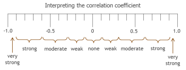
Are correlations on the rise?
B.33 There are several reasons why worldwide investment return correlations are tending to move together more than in the past. One cause for gradually rising correlation between markets over time is globalisation. Globalisation has increased the interrelation of the world's economies, internationalised investment flows, and
concentrated liquidity into a few major exchanges. A second cause is that volatility itself, being a parameter in asset option valuation, is now tradeable on financial exchanges, and heightened fear can lead to heavy trading in volatility (e.g. the VIX) and so to greater synchronised market volatility.
B.34 Increased market correlations have been observed both when the market is rising and
also in periods of market stress[3]. When markets rise and fall together, some of the benefits of diversification found in normal market conditions disappear. One cause of sudden, high worldwide correlation is spill over from a major market. For example, high volatility in the US tends to be associated with high volatility in non-US markets. When the US stock market crashed by 20 per cent in October 1987, the UK, Japanese and German markets fell at the same time, between 8 and 15 times their daily average variation.
B.35 Once ordinary conditions return, correlations tend to decrease. This suggests that the
benefits of diversification across asset classes and markets can reduce when they're needed most, such as in times of stress and market collapse. A very low risk approach that mixes low correlated assets will reduce this potential source of volatility.
Domestic or international investment?
B.36 A further aspect to consider is domestic or international investment. In recent times
the portfolio costs of investing internationally have fallen and are now not significantly more than investing domestically. This makes overseas investments potentially important to consider.
B.37 Evidence suggests that diversification over issuers of securities, maturities, industries
and countries will reduce risk further without necessarily sacrificing returns. Diversifying in all of the ways above will reduce the specific risk of investments and instruments and result in a portfolio with lower market risk than is possible if diversification is only partially applied. Based on this, the expectation has to be that an investor will seek to improve the risk and return trade-off through diversification across asset classes, markets and industries. Presuming this, for a very low risk investor, World equity, World bonds, and World government inflation linked bonds can be seen to be more appropriate assets than domestic, UK only, assets.
The level of diversification within an asset class, investment charges and taxes
B.38 To represent the investment performance of each asset class diversified indices have
been used. A diversified index for an asset class reflects the performance to an investor who invests across a broad set of securities so that they're only subject to the systematic, undiversifiable, risk of the asset class. For example, a world equity index will comprise several thousand company names from around the World. The indices selected are from highly regarded data sources and chosen because they have the longest data histories available for each asset class.
B.39 Fund managers can establish funds for investors that replicate these indices. This leads to transaction costs involved in maintaining close correspondence with the
index, and management costs and charges. To correct for this the analysis deducts 100 basis points, or 1%, from the annual performance of each bond index as an estimate of the after cost performance and 1.25% annually from each equity index. This includes an allowance for tax. We appreciate that broad brush allowance is only an approximation to the likely impact on investment returns of taxation and management expenses, but time constraints have not permitted a more detailed study of this issue.
B.40 The investor will normally access the chosen assets in the form of funds, or indeed
funds of funds. For example, the performance of a UK corporate bond index will be obtained by the investor choosing a fund manager's UK corporate bond fund.
Section C: The investment risk characteristics of the assets separately Introduction
C.1 The aim of this section is to analyse the investment risk of the assets separately and
their appropriateness for a very low risk investor. The analysis will look at:
• Variability of investment returns below inflation.
• Severity of drops from high to low in market value.
• Sequencing of investment return risk.
• Variability of inflation adjusted returns.
C.2 Assets found not to be individually appropriate or with an available and better
alternative are excluded and not used in the construction of the investment portfolio that follows.
C.3 In general the charts presented below will indicate that:
• Equities are higher risk but also higher return. Their use in a mixed portfolio for a low risk investor is based on their having strong risk diversification and a positive correlation to UK inflation.
• Corporate bonds have provided significantly more investment return than ILGS for more or less the same variability in market value about RPI. UK corporate bonds do not have a long data history but their low downside risk and correlation to other asset classes suggest a potentially significant role in a low risk portfolio. One concern in this respect is that bond markets in general have been in a secular bull market for very many years, and future returns, in absolute terms or relative to other assets, may be unpredictable. Central bankers have in fact expressed concerns over a turn' in the bond markets and its wider consequences in recent weeks.
• UK Treasury Bills have tracked RPI the closest over time, but with returns often slightly below RPI after deducting costs, charges and taxes of 1% per annum.
• World government inflation linked bonds have provided significantly more investment return than ILGS for slightly more variability in market value about RPI.
• ILGS have produced the lowest investment return per unit of downside risk over time. ILGS have the worst sequencing risk of below RPI returns. This comment, and the analysis that follows, relates to holding period returns from ILGS which are impacted upon by movements in yields in the market. An investor purchasing ILGS and holding them to redemption is guaranteed the yield secured at the time of purchase, there is no risk and the return, relative to inflation, is known in advance.
• Government bonds are generally more prone to long sequences of below RPI investment returns and greater peak to trough drops in market value than equities.
• Investing internationally increases diversification and lowers risk for similar return. It's the right course for a very low risk investor. For example, the World equity index has had less investment risk relative to RPI than the UK equity index, and the World government bond index has been less variable than a UK Gilt index.
C.4 The following eight charts present the investment risk and return of the assets relative to RPI. The evidence in the charts will be used to further exclude some types of asset.
Chart 1
C.5 Chart one presents the annualised risk and real return for the assets over their 115 year
history, or since inception. Investment returns are real, average annual returns after deducting an estimate of management costs and charges[4]. Risk is the standard deviation of real annual investment returns.
 What is standard deviation?
Standard deviation is a standardised measure of investment return variability that reports downside and upside variability together as one number. Standard deviation tells us how tightly the investment returns are clustered around the mean value. When the investment returns are spread apart the standard deviation is larger. When the investment returns are tightly bunched together the standard deviation is smaller.
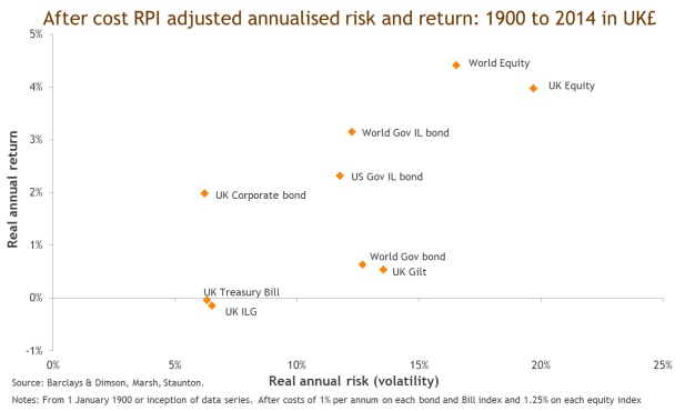
C.6 Chart 1 highlights:
• The long-run superior returns from equity investments that have been available in return for higher risk. This is to be expected in a rationally priced market, the excess return is the reward' for taking risk, which can also mean loss of capital.
• That diversification by country has generated lower risk for similar return. For example, the World equity index has been less variable than the UK equity index, as has the World government bond index compared to the UK Gilt index.
Chart 2
C.7 Chart 2 presents downside and upside variability about the average value. On the y-
axis, zero is RPI. The bars therefore show how close the investment returns of each asset have tracked RPI over time. The bars present the 95th to 5th percentile range of investment returns for the asset classes. This is the range of investment returns one
can expect 90% of the time (95% - 5% = 90%), or 9 out of each 10 years. The left panel shows the whole data history of each asset class, the right panel shows only the range of investment returns since 1999. This takes in the dotcom bust and financial crisis. 1999 has been chosen as this is the inception of UK corporate bond data.
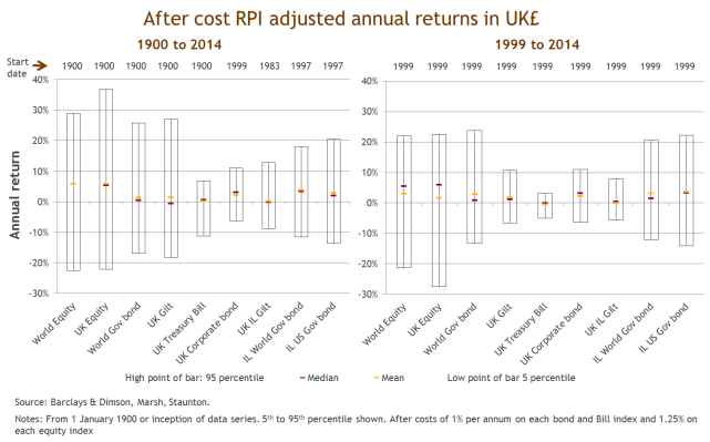
C.8 Chart 2 indicates that:
• Equities are a relatively high risk investment. Investors tolerate higher risk only if they believe better returns are on offer.
• Investing internationally has provided lower long-run investment risk. World equity and World government bonds have a narrower spread of investment returns relative to RPI than UK equities and bonds over the whole history (left panel).
• Treasury Bills track RPI the closest of all the assets.
Chart 3
C.9 Chart 3 shows the tracking error of investment returns relative to RPI since 1983, as
1983 is the inception of UK ILGS data. Tracking error reports the spread of upside and downside investment returns relative to RPI together as one number – a standard deviation.
 What is tracking error?
Tracking error first of all takes each investment return minus RPI. One can think of this as how much each investment return is moving away from RPI. Having calculated how investment returns are moving in relation to RPI, tracking error takes the standard deviation of these movements. So tracking error takes at its starting point that the riskiness of an asset is determined by measuring it relative to RPI.
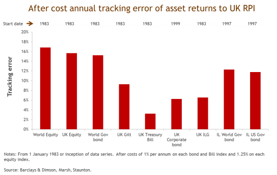
C.10 Chart 3 has shown that:
• Equities have tracked RPI least closely over time.
• UK Treasury Bills have tracked RPI most closely over time.
• Corporate bonds and ILGS have tracked RPI as well as each other over time, when considering holding period returns. As discussed above, if held to redemption, ILGS guarantee the return available at the time of purchase.
• UK Gilts have tracked RPI more closely than World government bonds.
• While tracking error looks at upside and downside variability together, intuitively downside risk is more concerning than upside risk for a very low risk investor. Based on this, the remaining charts focus only on investment returns below RPI.
Chart 4
C.11 The left panel of Chart 4 illustrates how tight or spread out investment returns are
below RPI for each asset as a standard deviation, so shows investment risk below RPI. This is known as semivariance. Any variability of investment returns above RPI are not part of the calculation.
The right panel of Chart 4 shows the long-run average annual investment return divided by the investment risk in the left panel, or the investment return earned per unit of downside (below RPI) risk. This is known as downside deviation. Chart 4 commences 1983, which is the start of the data history for ILGS.
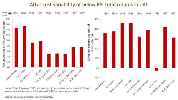
C.12 Chart four illustrates the following:
• Equities have the highest downside investment risk (left panel).
• UK Treasury Bills, and corporate bonds have similar below RPI investment risk (left panel).
• World equities and World government bonds have had less downside risk than UK equities and Gilts (left panel).
• World government inflation linked bonds have provided relatively good investment returns per unit of downside investment risk (right panel).
• ILGS have produced the lowest investment return per unit of downside risk over time (right panel).
Chart 5
C.13 Chart 5 presents maximum real drawdown for the assets. Maximum drawdown is an
important metric of financial risk for investors concerned about preserving and protecting capital. Maximum drawdown measures the highest peak to lowest trough drop over the entire history of an asset and reports that as a percentage change. It shows how bad the drop in value can be if a person invested at the highest value ever and then sold at the lowest value reached in any subsequent cycle during the whole data history. The information conveyed is straightforward to interpret as it's the absolute value of capital lost.
 What is drawdown?
Drawdown measures the amount of capital lost due either to a sequence of falling returns or a single large drop. Drawdown calculates the drop from the highest peak value to the lowest trough value over a given time period of an investment and reports that as a percentage change. For example, 10 year drawdown measures the change from the highest peak in the data to the lowest trough during the 10 year period. A measurement of capital lost also points to the gain needed to recoup this. If a fund lost 75% of its capital, it needs to gain 300% just to break even.
Avoiding potential large drawdowns is especially important for: Low risk tolerant investors.
Investors managing to a future liability.
Investors drawing an income from a fund.
Investors contributing regular or irregular amounts to a fund – not applicable for a claimant investor who spends income and dissipates capital over the expected period of loss.
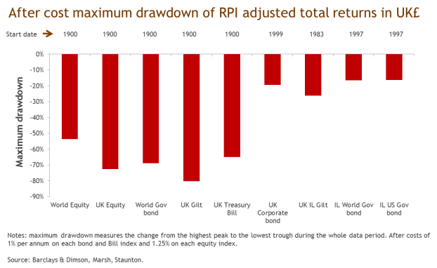
C.14 Chart 5 indicates that[5]:
• Corporate bonds have had low maximum drawdown.
• UK Treasury Bills, World government bonds and UK Gilts suffer from long sequences of low to moderate investment returns below RPI. This has led to large drawdowns.
• ILGS have had a larger maximum drawdown than UK corporate bonds and World government inflation linked bonds. This does not apply if held to redemption.
Chart 6
C.15 Chart 6 presents calendar 10 year drawdowns starting from 1970. This shows the
impact of economic shocks and market regimes on peak to trough drops in the market value of assets. Clearly visible is the 1970s oil crisis, the bursting of the dotcom bubble, and financial crisis between 2000 and 2009.
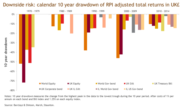
C.16 Chart 6 highlights:
• There can be significant drawdowns even among asset classes known for being relatively cautious investments, for example UK Gilts and UK Treasury Bills,
C.17 The final investment risk looked at is sequencing risk. Sequence of returns risk is the
risk of receiving a succession of below RPI investment returns. One of the lessons of the technology boom and bust followed shortly by the financial crisis was the importance of the order, or sequence, of extreme investment returns.
Chart 7
C.18 Chart 7 presents the number of sequences of below RPI investment returns and their
persistence. Sequencing risk occurs where one year of below RPI investment returns is immediately followed by another, which is immediately followed by another etc. This is shown by the length of the bars. Within the bars the number of times a particular sequence of below RPI investment returns was repeated during the data history is reported.
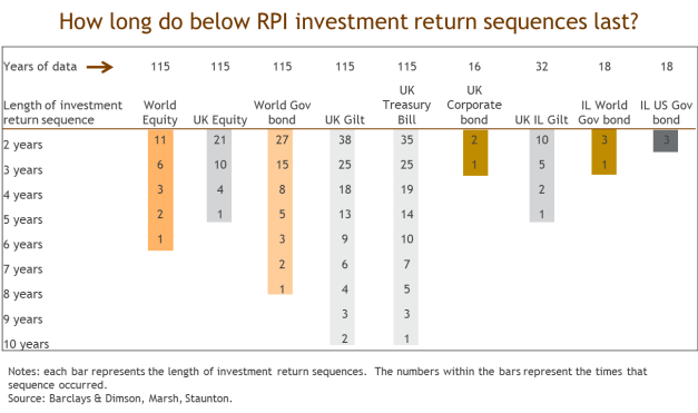
C.19 Chart 7 indicates the following:
• Equities have had less sequencing risk than bonds. They're not high sequencing risk.
• UK Gilts and Treasury Bills have had 10 year sequences of below inflation returns. This makes them more risky on a mark-to-market basis than one might imagine. Investment returns are often below RPI and bunched.
• ILGS have a relatively short, 32 year trading history, but already there is one five year sequence of below RPI holding period investment returns.
 How relevant is sequence of return risk?
A good illustration of how important sequence of investment return risk can be is the
 early to mid 1980s. The chart below presents four 25 year world equity return histories, each 1 calendar year apart from the other. One person investing in 1982 experienced a quite different set of investment returns from a person investing in 1983 or 1984. Although each of the four 25 year lines started just one year apart from the other, after 25 years total investment returns are 100% different. So the period of investment only has to alter slightly for entirely different financial outcomes to occur.
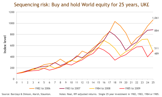
The example above is for a rising market, but poor investment return sequences can combine with portfolio withdrawals in a highly destructive way because more fund units need to be enchased to generate the same annual income. There is a double erosion of capital following a market fall – the market drop and the drawing an equal income at depressed fund value. The popular financial press refer to this scenario as pound cost ravaging'.
Chart 8
C.20 Chart 8 shows one more aspect of sequencing risk. Presented is the ratio of below RPI
investment return sequences that did occur over time relative to those that could have in theory occurred given the length of the data:
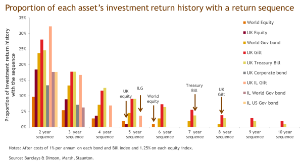
C.21 Chart 8 highlights that:
• ILGS have had the highest 2 year sequencing risk but only if holding period returns are being considered.
• Looking across all the years, ILGS, UK Gilts, Treasury Bills, and World Government Bonds have the highest sequencing risk.
• Equities have had relatively low sequencing risk.
• Below inflation annual investment returns that do not have long sequences or aren't closely bunched are more easily managed from a portfolio construction perspective through diversification and asset allocation. When there are long sequences of below inflation returns or closely bunched shorter sequences it's more difficult to manage from a portfolio construction perspective – one investor may be unlucky and experience a long sequence of below inflation returns or closely bunched shorter sequences while another investor may get lucky and encounter only above inflation returns.
Conclusion
C.22 The analysis has indicated that the assets below have better alternatives:
Assets with better available alternatives | |
Asset | Reason |
UK equities | Not as diversified or low risk (relative to RPI) as World equities. |
UK Treasury Bills | Best at tracking RPI but prone to significant sequencing risk and peak to trough drops in value over time. |
UK Gilts | Not as diversified or low risk (relative to RPI) as World government bonds, prone to significant sequencing risk and peak to trough drops in value over time. |
US government inflation linked bonds | Not as diversified or low risk (relative to RPI) as World government inflation linked bonds. |
C.23 As the assets above have better available alternatives they're discontinued and not
used as possible building blocks to construct a portfolio consistent with the investment risk objective. The assets that remain right for the investor after this analysis and considered in the construction of a very low risk investment portfolio are as follows:
Assets to be used in the portfolio construction | |
Asset | Reason |
World equities | A diversified index with relatively low sequencing risk that's correlated with inflation but with low correlation to the other assets. |
UK corporate bonds | A strong diversifier that has tracked RPI quite closely with above RPI investment returns. There has been low sequencing risk and peak to trough drops in value. |
World government bonds | A diversified index with moderate correlation to the other assets and low to moderate investment risk across the 8 charts and metrics analysed in Section Three. |
World government inflation linked bonds | A diversified index with lowish correlation to the other assets and lowish investment risk across the 8 charts and metrics analysed in Section C. There has been lowish sequencing risk and peak to trough drops in value. |
ILGS | The real risk free rate and a strong diversifier that has low correlation to other assets. ILGS offer very poor mark-to- market total returns for their level of investment risk and the optimiser may exclude these in the best low risk portfolio. |
Section D: Modern Portfolio Theory – combining a mix of investments to achieve a very low risk investment portfolio
D.1 In this section portfolios are constructed from the following assets that Section C
suggests are potentially appropriate building block assets:
• World equities
• UK corporate bonds
• World government bonds
• World government inflation linked bonds
• ILGS
D.2 A set of efficient, low correlated, diversified portfolios are identified. From these an
optimal mix of risky investments is identified as the "best risk portfolio". Results suggest that even the investment risk of the optimally constructed portfolio is likely to exceed the risk tolerance of a very low risk investor.
D.3 The solution to the risk tolerance problem may be to combine the risk free/market
consistent approach in Chapter 1, in which it's assumed that the yield on ILGS is the real risk-free rate and that ILGS are bought and held to maturity (so ignoring mark-to- market total returns), with a financial economics mark-to-market, fair value, total return approach in which a mix of risky investments are held[6]. The hypothetical claimant invests some money into ILGS and some into the optimal mix of risky investments. This is called the "best risk portfolio". Only a fraction is invested into the best risk portfolio. This technique is known as the two fund separation theorem and is a standard approach to asset allocation for investors within Modern Portfolio Theory. The best risk portfolio comprises 50% UK corporate bonds, 30% World government inflation linked bonds, and 20% World equities. By investing one-half in the best risk portfolio and one-half in ILGS, the investment risk taken is halved, compared to the optimally constructed risky portfolio. By investing one-quarter in the best risk portfolio and three-quarters in ILGS, the investment risk taken is one- quarter, compared to the optimally constructed risky portfolio. Although what level of risk might be deemed to be very low' will vary between investors these two selected portfolios may be considered to be consistent with a very low investment risk tolerance in real terms. The long-run real expected investment return is then read off.
D.4 The first of the two portfolios has 50% of the investments in ILGS (presumed to have
no risk), 25% in corporate bonds, 15% in overseas developed country government inflation linked bonds, and 10% in equities. The expected long-run annual real investment return on this first portfolio is:
Asset | Portfolio weight (%) | Portfolio return (%) |
Risk free/ILGS | 50 | -1.0% 1 |
Corporate bonds (25%), Overseas developed country government inflation linked bonds (15%), Equities (10%) | 50 | 2.50% |
1 this is current after tax real yield on ILGS, from Chapter 1 | ||
D.5 The expected investment return is (50% x -1.0%) + (50% x 2.5%) = 0.75%, rounded
to either 0.5% or 1% depending on one's policy in this regard.
D.6 The second portfolio has 75% of the investments in ILGS (presumed to have no risk),
12.5% in corporate bonds, 7.5% in overseas developed country government inflation linked bonds, and 5% in equities. The expected long-run annual real investment return on this second portfolio is:
Asset | Portfolio weight (%) | Portfolio return (%) |
Risk free/ILGS | 75 | -1.0% 1 |
Corporate bonds (12.5%), Overseas developed country government inflation linked bonds (7.5%), Equities (5%) | 25 | 2.50% |
1 this is the rounded ILGS return from Chapter 1 | ||
D.7 The expected investment return is (75% x -1.0%) + (25% x 2.5%) = -0.125%,
rounded to 0%.
D.8 In this section a mean variance optimisation is performed and the efficient frontier
found. Along the frontier efficient portfolios are located. We're interested in the efficient portfolios with a low dispersion of real investment returns.
D.9 Five charts are now used to derive the best risk diversified portfolio and present its
investment risk and return relative to RPI.
 The efficient frontier and mean variance optimisation What is the efficient frontier?
 The shaded region – or cloud, on the illustration below corresponds to the achievable risk-return space of the assets. For every point in that region, there will be at least one portfolio that can be constructed that has levels of risk and return corresponding to that point. The efficient frontier is the purple curve that runs along the top of the achievable region. It is used as the standard approach to asset allocation.
The efficient frontier is the set of investment portfolios which meet the following conditions:
Offer maximum expected return for varying levels of risk.
Offer minimum risk for varying levels of expected return.
The preferred portfolio will correspond to the point on the efficient frontier which represents the risk the investor is prepared to tolerate.
The portfolios further to the top right of the efficient frontier tend to be portfolios with high weightings in equities. The portfolios further to the bottom left of the efficient frontier tend to be portfolios that mix assets with low co-movement to one another, for example bonds and equities.
If no point satisfies the risk that the investor is prepared to tolerate the solution is to put some money in the best risky portfolio on the efficient frontier and some in the risk free asset. The risk free asset is assumed to have no investment risk – systematic or unsystematic.
How to find the efficient frontier?
In order to find the efficient frontier for the assets and so the investment allocation consistent with the risk objective, the first step is to assess the annual return for each of the assets, their volatility, and a measure of the correlation between them. The efficient frontier can then be plotted using an optimisation process. This is known as mean variance optimisation'.
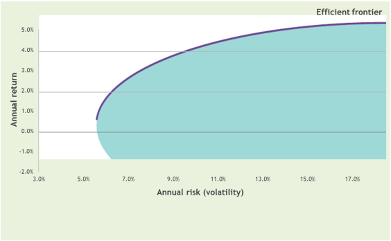
Chart 9
D.10 Chart 9 presents the efficient frontier for the assets from the mean variance
optimisation. Along the efficient frontier are located efficient portfolios in terms of their investment risk and return combination. Below the efficient frontier lie a cloud of other portfolios (not shown) that didn't meet the optimal conditions needed to lie on the efficient frontier. The individual assets are in this cloud, and are included in the chart for information. Data are after costs and real, RPI adjusted.
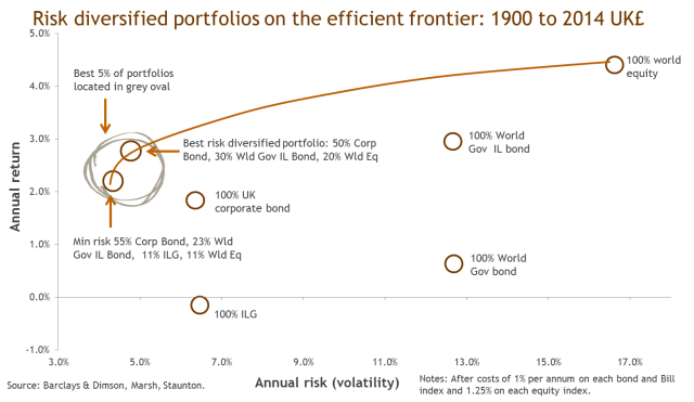
D.11 Chart 9 shows the position of the efficient frontier. On that frontier 2 fully invested
investment portfolios are pulled-out as being of most interest. These are:
• The minimum risk portfolio – real risk of 4.5%, real return of 2.2%.
• The best risk portfolio – this has the highest return per unit of risk (Sharpe ratio), so is superior to the minimum risk portfolio in terms of return per unit of risk taken. This has real risk of 5.0%, real return of 2.8%.
• This is the long-run picture, going back a long time.
D.12 Chart 9 indicates:
• The significant risk diversification had from assembling the assets into mixed investment portfolios. They're to the left of the risk-return combinations of the individual assets.
• The location of the best 5% of portfolios according to the amount of investment return obtained per unit of risk taken (Sharpe ratio).
• The very lowest risk portfolio on the efficient frontier contains 55% UK corporate bonds, 23% World government inflation linked bonds, 11% ILGS, and 11% World equities.
• The portfolio with the highest investment return per unit of risk – the best risk portfolio, comprises 50% UK corporate bonds, 30% World government inflation linked bonds, and 20% World equities.
Chart 10
D.13 Chart 10 presents the distribution of returns for the minimum risk portfolio and the
best risk portfolio on the efficient frontier.
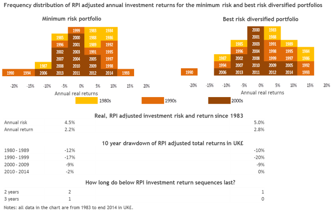
D.14 Chart 10 shows:
• That both the minimum risk portfolio and the best risk portfolio (the one with the higher Sharpe ratio) have similar downside risk. The left side of each distribution looks fairly similar. If anything, the minimum risk portfolio has more downside risk because of more downside sequencing risk.
• The best risk portfolio is virtually sequencing risk free, while the minimum risk portfolio is not.
• There is no significant difference in the drawdowns of either portfolio.
• The small extra volatility of 0.5% contained in the best risk diversified portfolio is therefore upside volatility – more mass can be seen in the right side of the distribution compared to the minimum risk portfolio.
• The best risk diversified portfolio is the better portfolio to select. This is the standard approach in theory and in practice – the minimum risk portfolio is usually not the best risk portfolio and is rejected in portfolio construction.
D.15 Looking at the best risk portfolio in Chart 10, one cannot say that the portfolio is
consistent with a very low risk investment objective. The frequency distribution of annual returns contains a left tail that has too much investment risk for a very low risk appetite. Calendar 10 year drawdowns – or peak to trough drops in market value, remain too high for a very low risk appetite. In short, the mean variance optimisation' has not been able to generate a 100% mixed risky investment with low enough risk.
D.16 The solution is for the investor to put some money in the best risk portfolio and some
in ILGS, which are assumed in this report to be the closest there is to a risk free rate – provided they're bought and held to maturity. The linear combinations of the two investments are shown in Chart eleven.
Chart 11
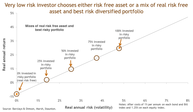
D.17 Chart 11 highlights that:
• Assuming that ILGS are virtually investment risk free, an investor with a very low appetite for risk will find an appropriate combination of ILGS and the optimal mix of risky investments.
• A very low risk investor might put one-half, 50%, into ILGS and one-half into the best risk portfolio, or three-quarters, 75%, into ILGS and one-quarter into the best risk portfolio.
• When only 50% is invested in the best risk portfolio all the investment metrics in Chart 10 are halved, and the frequency distribution of investment returns becomes much tighter, as shown in Chart 12.
Chart 12

D.18 In Chart 12 the mass of distribution of annual returns is in the middle with equal mass
in the shoulders of the distribution. The distribution has virtually no skewness (-0.17) and zero excess kurtosis (0.01). There is some very limited, but probably tolerable, left tail risk.
Use data from 1999 to set the discount rate from a financial economics perspective
D.19 Arguably the better approach would be to use the performance data starting in 1999
when considering expected investment returns and setting the discount rate. This is because UK corporate bond data begins in 1999. From 1983 to 1999 the best risk diversified portfolio does not contain any corporate bonds at all - it can't. From 1999 the best risk diversified portfolio does contain corporate bonds and that's why the frequency distribution of returns is tighter from 1999 to 2014. From 1999 all assets are available, diversification is strongest, and the best risk portfolio is at its most efficient.
D.20 From 1st Jan 1999 to end Dec 2014 the best risk portfolio has real annual risk of 5.0%
and real annual return of 2.5%. Chart 13 shows the key investment risk metrics since 1999 for a very low risk tolerant investor:
Chart 13
Investment risk according to proportion held in the best risk portfolio
Proportion of risky portfolio held
100% 50% 25%
Investment return and volatility
Annual average return above RPI 2.5% 1.25% 0.625% Standard deviation (volatilty) of returns 5.0% 2.50% 1.25%
Five key investment risk metrics most relevant to the Prime Directive
- Downside volatilitybelow RPI 2.5% 1.3% 0.6%
- 95% Value at Risk -5.3% -2.7% -1.3%
- 5% Conditional Value at Risk -7.0% -3.5% -1.8%
- Drawdown
4a. Drawdown 2000t 2009 -8.8% -4.4% -2.2% 4b. Drawdown 2010t 2014 -0.2% -0.1% 0.0% 4c. Max drawdown 1999t 2014 -8.8% -4.4% -2.2%
- Sequencingrisk virtually 0 virtually 0 virtually 0 Notes: RPI averages 2.85% between1999and 2014.
D.21 The risk measures in Chart 13 are the most relevant to the Prime Directive. D.22 According to Chart 13:
• The best risk portfolio has no sequencing of investment return risk.
• The real, RPI adjusted, 95% Value at Risk is low. This is the expected return 1 in 20 years and is -2.7% real when the hypothetical claimant invests one-half in the best risk portfolio, and -1.3% real when the hypothetical claimant invests one-quarter in the best risk portfolio.
 What is Value at Risk (VaR)?
Value at Risk (VaR) reports the per cent of capital, or fund value, that's expected to be lost at a given probability level. The probability level of 95% gives an estimate of the value lost at the threshold where 95% of investment returns will be better but 5% worse. So if an investor has a 20 year investment time horizon, 95% VaR tells the investor the loss that is likely 1 year in every 20. The investor can then decide their comfort level. The main drawback is that VaR is only the amount which is at risk with a particular probability. For example, it doesn't say what's likely within the worst 5% of investment returns.
D.23 The real, RPI adjusted 5% Conditional Value at Risk (CVaR) remains low. CVaR
indicates extreme left, or downside, tail risk. CVaR is -3.5% real when the hypothetical claimant invests one-half in the best risk portfolio, and -1.8% real when the hypothetical claimant invests one-quarter in the best risk portfolio.
 What is Conditional Value at Risk (CVaR)?
CVaR addresses the drawback of VaR just noted. CVaR is the average, or mean, investment return on the portfolio in the worst 5% of the cases. It is a measure of tail risk' and focused on the very worst investment outcomes. CVaR tells us "if I do end up in the tail of the 5% of worst investment return outcomes, what is the average loss I will incur (the mean loss in the 5th to 0 percentile)?"
D.24 The low volatility, low VaR, CVaR, low peak to trough to trough drops in market
value and no sequencing risk all support an investment allocation of either 50% or 25% in the best risk portfolio.
D.25 The other part of the investment is made in ILGS and receives the yield on this. If the
tail risk (CVaR) noted above materialised, and 50% was invested in the best risk portfolio, the real portfolio return would be -3.5% plus the investment return obtained on the 50% invested in ILGS of -0.5%. This tail risk case scenario of -4.0%, is slightly less than average RPI of 2.9%, and suggests in that particular year a nominal portfolio return of about -1.1%.
D.26 Chart 14 shows the money and risk weights for the best risk portfolio. Chart 14
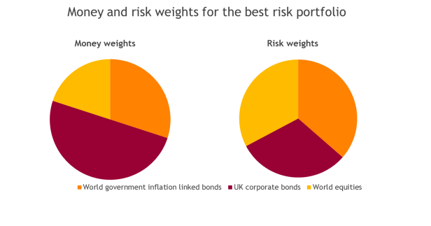
D.27 Chart 14 indicates:
• The best risk portfolio is equally balanced in terms of the partial contribution to portfolio risk from corporate bonds, equity, and world government inflation linked bonds (right pie). This is the result of the mean variance optimisation, which seeks to maximise diversification.
• The best risk portfolio is more diversified than would be suggested by looking only at the money weights (left pie). Less money is put into equities because it's a more risky investment. The low money weight x the higher investment risk of equities = the equity risk weight.
• More equal risk allocation is likely to provide more consistent performance in different market regimes.
Limitations
D.28 The study is not without limitations. The following are the major ones to note.
D.29 The mean variance optimisation is limited by the quality of the information used to
generate the achievable risk return space. If the data about the expected return and risk of different assets are poor, the optimal mix of risky investments may be inappropriate.
D.30 By using long data histories of actual historic returns as they occurred in sequence
we're assuming that the future will sometimes echo the past, and that there is some value in examining past data as a guide to the sorts of things we can expect over time. There are other approaches. These include sampling techniques based on created distributions or drawing on forward-looking capital market assumptions data. All approaches have their merits, but this approach is to look back 115 years.
D.31 The investments considered have been liquid, long only, without leverage, hedging, or
use of derivatives.
D.32 The investor is assumed to invest independently or through an adviser. The resident country is assumed to be the UK so all analysis is in UK£. The investor is long-term
and interested in real investment risk and return. All the analysis is in real, RPI adjusted, terms. The Retail Price Index (RPI) is the chosen inflation index for the reasons outlined in Chapter 3.
Triggers for review
A3.1 Events that might trigger a future review of the discount rate are:
A3.2 In the event the discount rate is set by reference to ILGS yields alone:
• A material change in the redemption yields on ILGS. On the assumption that the discount rate continues to be set as a multiple of 0.5% we would suggest that the moving one year average of over 5 year yields be monitored and consideration given to changing the discount rate when this moves into a higher or lower band than at the time the rate was last set.
• The issuance of CPI-linked government stocks.
• A material change in taxation levels and rates.
A3.3 In the event that the discount rate is not set by reference to ILGS yields alone, one
should also consider:
• A material change in expected real investment returns.
• A material change in expected real investment risk.
• A material change in security availability and investment liquidity.
• A material change in investment costs and charges.
• Modest changes in a number of the above that lead to an overall material change.